AI Model Structures - 25
Welcome,
Let’s take a look at the history of The Model Structures we’re using today.
1. Why「Deep Structure」
Compared with the original machine learning models:
- Linear Regression / SVM / Shallow Decision Trees
Deep structures refer to neural networks with Multiple Layers of Nonlinear Transformations
📍 Content
- Transformer
- BERT
- Mamba
- GPT
- Tokenization
- ARIMA
- RNN
- Diffusion Models
- Flow Matching
- TensorRT
- Quantization - LoRA + QLoRA 📍
These deep models are capable of Learning Hierarchical Features, where each layer captures increasingly abstract representations of the data.
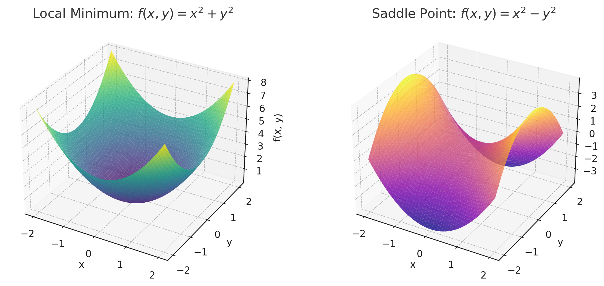
Local Minimal vs. Saddle Point
In practice, “Deep” means:
-
More than 3–4 layers in fully connected networks
-
10+ layers in convolutional networks
-
Or even hundreds of layers in modern transformers like GPT and BERT
2. Key Tech
-
MLP
- Multilayer Perceptron
- Feedforward fully connected networks
- Used in classification, regression, or small-scale tabular/audio tasks
- 1989 - Universal Approximation Theorem / Still used as light head in multimodal systems
-
RNN -> LSTM
- When inputs are sequences
-
Hochreiter & Schmidhuber 1997 - LSTM
- When inputs are sequences
-
CNN
- Convolutional Neural Networks
- When inputs are images or grid-like data
- Extracts spatial features, widely used in image/audio tasks
- Fully Connected Layer -> Receptive Field -> Parameter Sharing -> Convolutional Layer
- 1998 - LeNet / 2012 - AlexNet: ImageNet Classification with Deep Convolutional Neural Networks
-
Transformer
- When inputs are sequences
- Self-attention + Parallel computation
-
2015 ICLR - Neural Machine Translation by Jointly Learning to Align and Translate - Additive Attention
-
2017 NeuralPS - Attention Is All You Need - Self-Attention / Scaled Dot-Product Attention
- When inputs are sequences
-
📍 Mamba
- Linear-Time Sequence Modeling
- State Space Model - SSM - with selective long-range memory
-
2023 - Mamba: Linear-Time Sequence Modeling with Selective State Spaces
- Linear-Time Sequence Modeling
-
BERT
- Bidirectional Encoder Representations from Transformers
- using Masked language modeling
-
2019 - BERT: Pre-training of Deep Bidirectional Transformers for Language Understanding
- Bidirectional Encoder Representations from Transformers
-
Conformer
- Convolution + Transformer = Conformer
- Combines local - CNN - and Global Self-attention Features
- Widely used in speech recognition tasks
-
2020 - Conformer: Convolution-augmented Transformer for Speech Recognition
-
GAN
- Generator vs Discriminator
- Generates Images, Audio
- Popular in TTS, audio enhancement, and image generation
-
2014 - Generative Adversarial Nets
- Generator vs Discriminator
-
Diffusion Based
- Gradual denoising process to generate samples from noise
- Currently SoTA in image and speech generation
- Training is stable, generation is slow
-
In Diffusion
- The model learns to reverse noise through a pre-defined noise schedule
- It does not evaluate or penalize each intermediate step
- There is no “fitness score” like in genetic algorithms
-
In genetic algorithms - GA
- Every candidate (individual) is evaluated using a fitness function
- Poor candidates are penalized or discarded
-
2020 - Denoising Diffusion Probabilistic Models
- Gradual denoising process to generate samples from noise
-
📍 SSL
- Learns from unlabeled data by solving pretext tasks
- Strong performance in low-resource and zero-shot setups
-
2020 - wav2vec 2.0: A Framework for Self-Supervised Learning of Speech Representations
- Learns from unlabeled data by solving pretext tasks
-
📍 MEMORY - Transformers vs. RNN / LSTM
-
Add Reflection - 2024 - You Only Cache Once: Decoder-Decoder Architectures for Language Models
- RetNet - Retention Network -> Gated Retention
- 2023 - RetNet: Retinal Disease Detection using Convolutional Neural Network
- DeltaNet - 2025 - Parallelizing Linear Transformers with the Delta Rule over Sequence Length
-
Add Reflection - 2024 - You Only Cache Once: Decoder-Decoder Architectures for Language Models
Deep Learning
1. Premise of Deep Learning
The premise of deep learning refers to the underlying assumptions and principles that explain why deep neural networks work and when they are effective:
-
Manifold / Smoothness Assumption: High-dimensional data (images, speech, text) often lie on a lower-dimensional manifold, and semantic changes are locally smooth → can be approximated by continuous functions
-
Distributed & Hierarchical Representations: Complex concepts can be formed by hierarchical composition of features (edges → textures → objects)
-
Inductive Bias: Architectures like CNNs (translation equivariance) and Transformers (content-based selection) embed useful priors
-
Over-parameterization & SGD Implicit Regularization: Even with more parameters than samples, SGD tends to find “flat” minima that generalize well
-
i.i.d. and Distribution Stability: Training and test data should follow similar distributions, or be adapted via transfer learning/fine-tuning
-
Scalability (Scaling Laws): Increasing data, compute, and model size tends to yield predictable performance gains
Use cases: guiding architecture design, choosing regularization/data augmentation, understanding transfer learning, anticipating risks from domain shifts or small datasets
2. Word Embeddings
Word embeddings map discrete words into dense numerical vectors (usually 100–1024 dimensions) where geometric relationships capture semantic/grammatical similarity
-
Motivation: One-hot vectors are sparse and lack similarity information; embeddings allow “similar words” to be close in vector space
-
Classic methods:
- Word2Vec (CBOW / Skip-gram), GloVe – static embeddings from word co-occurrence
- FastText – includes subword n-grams to handle out-of-vocabulary words
- Contextual embeddings (BERT, LLMs) – same word can have different vectors depending on context
-
Similarity measure: cosine similarity
\[\cos = \frac{u \cdot v}{\|u\| \, \|v\|}\] - Applications: text classification, semantic search, clustering, recommendation, retrieval-augmented generation (RAG), cross-modal alignment (e.g., CLIP)
3. Dot Products
The dot product (inner product) between two vectors (a) and (b):
\[a \cdot b = \sum_i a_i b_i = \|a\| \, \|b\| \cos\theta\]- Geometric meaning: projection of one vector onto another, scaled by the first vector’s length
- Relation to cosine similarity: if vectors are normalized, dot product equals cosine similarity
-
Deep learning usage:
-
Attention scoring:
\[\text{score}_{ij} = \frac{q_i \cdot k_j}{\sqrt{d_k}}\] - Similarity in retrieval / contrastive learning (e.g., InfoNCE, CLIP)
- Final classification layer: logits as dot products between features and class weights
-
- Tip: often L2-normalize or apply scaling/temperature to control numerical stability
4. Softmax
The softmax function converts raw scores (logits) into probabilities:
\[\text{softmax}(z)_i = \frac{e^{z_i}}{\sum_j e^{z_j}}\]- Shift invariance: adding the same constant to all logits doesn’t change output
- Numerical stability: use
- Temperature scaling: (\tau < 1) → sharper distribution; (\tau > 1) → smoother
-
Gradient-friendly: with cross-entropy, gradients simplify to
softmax(z) - y -
Applications:
- multi-class classification output
- attention weight normalization
- contrastive learning normalization
- language model token sampling
Summary Connection
- Word embeddings: map words to vectors
- Dot product: measure similarity between embeddings
- Softmax: turn similarity scores into probabilities
- Premise of deep learning: explains why such representation + similarity + normalization pipelines work for large-scale AI tasks
4. Some Norms and Their Nature
CTC - Connectionist Temporal Classification - is a loss function used for sequence tasks where input and output lengths don’t match — like speech-to-text
- You don’t need exact alignment between audio frames and text
- CTC learns to map long input sequences (e.g. 1000 audio frames) to short outputs (e.g. “hello”)
- It introduces a special blank token - ∅ to allow flexible alignment
- The model can output repeated characters + blanks, and CTC will collapse them into the final label
– Input frames: [x1, x2, x3, x4, x5, x6, x7, x8] Model output: ∅ h ∅ e l l ∅ o CTC collapse: → “hello” –
📍 Why LSTM / other RNN Layer after Self-Attention Layer
- Streamability
- Positional bias
- Smoothing
- Lightweight after quantization
- Distillation bridge
- TLDR - Attention offers Global Context, the follow-up LSTM supplies Sequential Inertia, Latency Control, and Quantization-friendly compression—ideal for hearing-aid ASR
4. Some References
Enjoy Reading This Article?
Here are some more articles you might like to read next: