Model Structures - 25
- Let’s take a look at the history of the Model Structures we’re using today.
Evolution of 3D Scene Representations
| Period | Method | Representation | Advantages / Limitations |
|---|---|---|---|
| 1980–2010s | SfM / MVS / Mesh | Explicit point clouds or polygonal meshes | Accurate but discrete; cannot represent complex appearance or soft surfaces |
| 1990–2010s | IBR / Light Field | Sampled light rays or image interpolation | Highly photorealistic but lacks true 3D geometry; strong view dependence |
| 2015–2019 | Deep Implicit Fields | Implicit functions (Occupancy / Signed Distance Field) | Continuous and smooth geometry; no explicit color or reflectance modeling |
| 2020–2022 | NeRF family | Neural radiance fields (density + color) | Unified geometry and appearance; high fidelity but slow to train and render |
| 2023–Now | 3D Gaussian Splatting (3DGS) | Explicit point-based volumetric primitives (Gaussian ellipsoids with color, opacity, and anisotropy) | Extremely fast rendering and editing; preserves view consistency; but lacks strong geometry regularization and semantic understanding |
DL after Classic ML
| Component | Description |
|---|---|
| Origin | Deep Learning was formalized in 1986 by Rumelhart, Hinton, and Williams with the invention of Backpropagation. |
| Key Idea | Learn hierarchical representations — from low-level edges to high-level concepts — through multiple neural layers. |
| Representation | Automatically extracts features from raw data (images, audio, text) instead of manual feature engineering. |
| Optimization | Trains large neural networks using gradient descent and backpropagation to minimize a defined loss. |
| Architecture | Stacks multiple nonlinear transformations (e.g., CNNs, RNNs, Transformers) to form deep computational graphs. |
| Generalization | Learns robust patterns that transfer to unseen data, aided by large datasets, GPUs, and regularization methods. |
| Impact / Use | Powers modern AI systems in vision (CNNs), language (Transformers), speech (RNNs), and generative models (Diffusion, GANs). |
Deep Learning, Training, and Knowledge Distillation
| Dimension | Deep Learning | Training | Knowledge Distillation |
|---|---|---|---|
| Objective | Learn multi-layer nonlinear function f(x; θ) to represent complex patterns. | Optimize a loss function from data. | Make the student model mimic the teacher’s output distribution and internal representations. |
| Input Information | Raw data (x) | (x, y) | (x, y, T(x)) |
| Loss Function | Any differentiable objective. | Task loss 𝓛(f(x), y) | α 𝓛(f(x), y) + (1−α) KL(f(x) ∥ T(x)) |
| Supervision Source | Data itself. | Hard labels (y). | Teacher outputs (T(x)) + true labels (y). |
| Entropy Characteristic | May be high or low depending on task. | Low-entropy one-hot supervision. | High-entropy soft targets (smoothed teacher outputs). |
| Optimization Process | BP + GD (Backpropagation + Gradient Descent). | BP + GD. | BP + GD with temperature scaling τ. |
| Application Goal | General representation learning. | Task-specific model fitting. | Model compression, knowledge transfer, or performance enhancement. |
| Output Features | Deep hierarchical representations. | Task predictions. | Balanced task accuracy and teacher–student alignment. |
Deep Learning World                             Classical ML World
═══════════════════════════════════             ════════════════════════════════════
Raw Data → Multi-layer Network →                Handcrafted Features → Shallow Model →
Learn Representations → Optimize by Gradient    Manual Design → Limited Adaptability
     ↓                     ↓                           ↓                     ↓
┌───────────────┐   ┌─────────────────┐           ┌─────────────────┐   ┌───────────────────────┐
│ Raw Inputs    │ → │ Neural Layers   │    vs.    │ Engineered Feats│ → │ Classifier (SVM/Tree) │
│ (Image/Text)  │   │ (CNN/RNN/Trans.)│           │ (HOG/SIFT/MFCC) │   │ (Fixed Decision Rules) │
└───────────────┘   └─────────────────┘           └─────────────────┘   └───────────────────────┘
     ↓                     ↓                           ↓                     ↓
End-to-End Learning     Automatic Feature Hierarchy   Manual Tuning Needed   Poor Transferability
(Backprop + Gradient)   (Low→Mid→High Abstractions)   (Domain-Specific)      (Retrain for New Task)

Hybrid approaches:
1. Use pretrained deep features + classical models for fast adaptation
2. Fine-tune deep backbones with task-specific heads for efficiency

Deep Learning = Student who learns concepts from examples (automatic understanding)
Classical ML  = Student who uses fixed formulas (must be told what features matter)
Generalization Ability
Unsupervised World                              Zero-Shot World
═══════════════════════════════════             ════════════════════════════════════
No Labels → Discover Patterns →                 Pretrained Knowledge → New Task →
Cluster / Reduce Dim → Build Representations    Direct Prediction → Works Instantly
     ↓                     ↓                           ↓                     ↓
┌───────────────┐   ┌─────────────────┐           ┌─────────────────┐   ┌───────────────────────┐
│ Data Patterns │ → │ Learned Embeds  │    vs.    │ Language / Text │ → │ Recognize Unseen Task │
│ (Raw Inputs)  │   │ (Structure Only)│           │ Semantic Priors │   │ (Zero Examples)       │
└───────────────┘   └─────────────────┘           └─────────────────┘   └───────────────────────┘
     ↓                     ↓                           ↓                     ↓
Unclear for Tasks      Needs Extra Step            Direct Generalization   Immediate Usability
(PCA/K-means/SimCLR)   (Downstream Fine-tune)      (CLIP, GPT)             (Zero-shot QA/CLS)

Hybrid approaches:
1. Learn unsupervised embeddings → map to semantic space for zero-shot transfer
2. Combine raw pattern discovery with pretrained knowledge for stronger generalization

Unsupervised = Tourist wandering a city with no map (discover zones by yourself)
Zero-Shot   = Tourist with a guidebook (instantly spot city hall & cathedral)
Why Deep Structure
- Compared with the original machine learning models:
- Linear Regression / SVM / Shallow Decision Trees
- Deep structures refer to neural networks with Multiple Layers of Nonlinear Transformations
- how to find some other temporal modeling way for the Non-linear Transformation?
Content
- Transformer
- Mamba
- GPT
- Tokenization
- ARIMA
- RNN, LSTM, GRU
- Diffusion Models
- Flow Matching
- Quantization / Adapter Guided - LoRA + QLoRA
- These deep models are capable of Learning Hierarchical Features, where each layer captures increasingly abstract representations of the data.
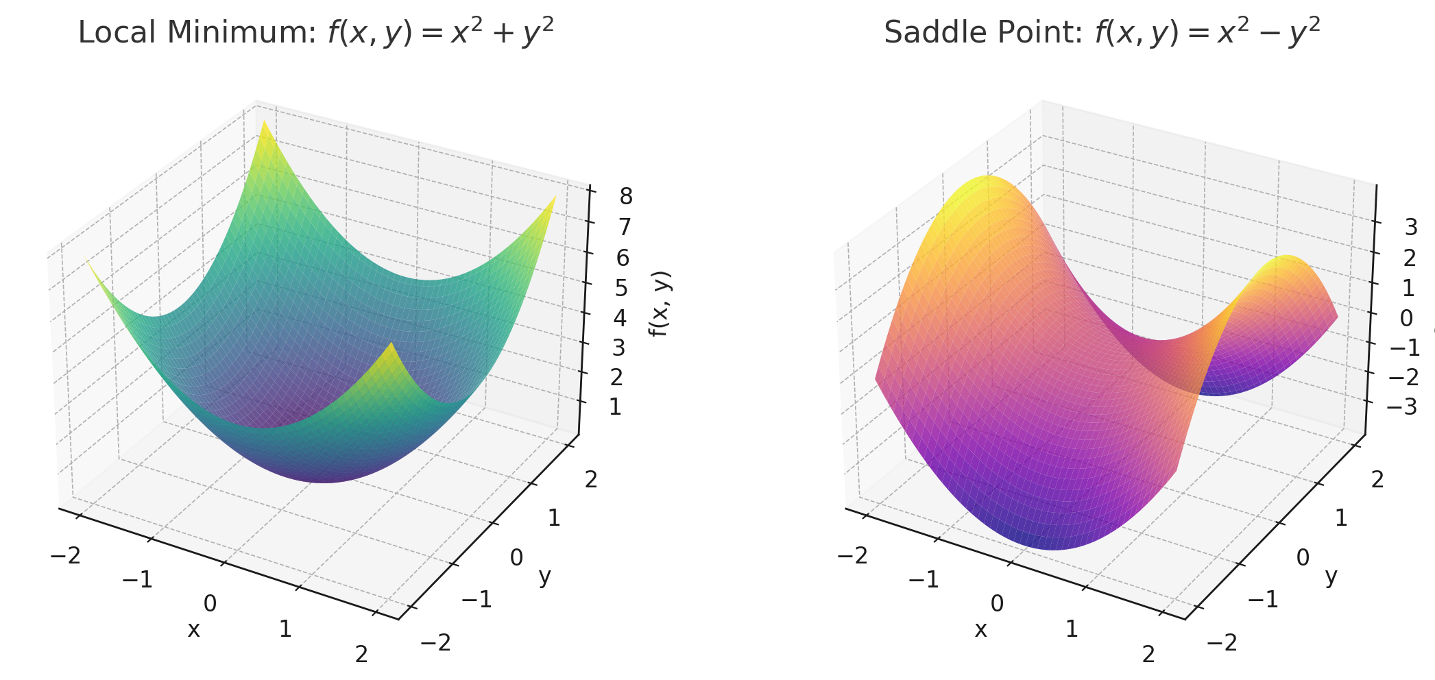
Local Minimal vs. Saddle Point
In practice, “Deep” means:
- More than 3–4 layers in fully connected networks
- 10+ layers in convolutional networks
- Or even hundreds of layers in modern transformers like GPT
Key Structures
- MLP
- Multilayer Perceptron
- Feedforward fully connected networks
- Used in classification, regression, or small-scale tabular/audio tasks
- 1989 - Universal Approximation Theorem / Still used as light head in multimodal systems
- 📍 RNN -> LSTM
- When inputs are sequences
- Hochreiter & Schmidhuber 1997 - LSTM
- When inputs are sequences
- Some Other 📍 Temporal Modeling
- GRU
- ConvGRU
- DynamicLSTM
- GatedGRU
- CNN
- Convolutional Neural Networks
- When inputs are images or grid-like data
- Extracts spatial features, widely used in image/audio tasks
- Fully Connected Layer -> Receptive Field -> Parameter Sharing -> Convolutional Layer
- 1998 - LeNet / 2012 - AlexNet: ImageNet Classification with Deep Convolutional Neural Networks
- Transformer
- When inputs are sequences
- Self-attention + Parallel computation
- 2015 ICLR - Neural Machine Translation by Jointly Learning to Align and Translate - Additive Attention
- 2017 NeuralPS - Attention Is All You Need - Self-Attention / Scaled Dot-Product Attention
- When inputs are sequences
- Mamba
- Linear-Time Sequence Modeling
- State Space Model - SSM - with selective long-range memory
- 2023 - Mamba: Linear-Time Sequence Modeling with Selective State Spaces
- Linear-Time Sequence Modeling
- Conformer
- Convolution + Transformer = Conformer
- Combines local - CNN - and Global Self-attention Features
- Widely used in speech recognition tasks
- 2020 - Conformer: Convolution-augmented Transformer for Speech Recognition
- GAN
- Generator vs Discriminator
- Generates Images, Audio
- Popular in TTS, audio enhancement, and image generation
- 2014 - Generative Adversarial Nets
- Generator vs Discriminator
- Diffusion Based
- Gradual denoising process to generate samples from noise
- Currently SoTA in image and speech generation
- Training is stable, generation is slow
- In Diffusion
- The model learns to reverse noise through a pre-defined noise schedule
- It does not evaluate or penalize each intermediate step
- There is no “fitness score” like in genetic algorithms
- In genetic algorithms - GA
- Every candidate (individual) is evaluated using a fitness function
- Poor candidates are penalized or discarded
- 2020 - Denoising Diffusion Probabilistic Models
- Gradual denoising process to generate samples from noise
- 📍 SSL
- Learns from unlabeled data by solving pretext tasks
- Strong performance in low-resource and zero-shot setups
- Learns from unlabeled data by solving pretext tasks
- Memory - Transformers vs. RNN / LSTM
- Add Reflection - 2024 - You Only Cache Once: Decoder-Decoder Architectures for Language Models
- Flow Matching
1. Gradient Noise
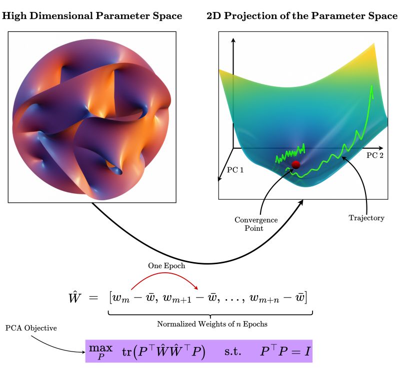
2. What is Gradient Noise
| Source | Explanation |
|---|---|
| Sampling noise | Each batch only samples part of the data, so the gradient is an approximation of the true mean. |
| Reward noise (RL-specific) | Rewards from the environment vary greatly across trajectories. |
| Numerical noise (hardware) | Floating-point rounding errors, limited bfloat16 precision, or non-deterministic accumulation order. |
| Communication noise (multi-GPU) | Random order of all-reduce operations causes slight variations in summed gradients. |
| Regularization noise | Dropout and mixed-precision scaling introduce artificial randomness. |
- Compute the exact gradient of the loss function (ideal case)
- Represent the noisy gradient observed in practice (with noise term ( \varepsilon ))
3. Why Gradient Noise is Especially Large in RL
\[J(\theta) = \mathbb{E}_{\tau \sim \pi_\theta}[R(\tau)]\]- Expected future reward objective in reinforcement learning
- Policy gradient estimating how parameters affect expected reward
- High variance of rewards and log-probabilities amplifies gradient noise
4. Learning Rates - Theoretically
5. Historical Development of Kernel Functions
| Year | Person / School | Contribution |
|---|---|---|
| 1909 | James Mercer | Proposed Mercer’s Theorem — the mathematical relationship between symmetric positive-definite kernel functions and inner-product spaces of high dimension. |
| 1930 – 1950 | Integral-Equation School | The term kernel originally referred to the weighting function of an integral operator, $K(x, y)$. |
| 1960s | Vapnik & Chervonenkis (USSR) | Developed statistical learning theory and introduced the idea of implicit feature mapping. |
| 1992 – 1995 | Vapnik, Boser, Guyon, Cortes | Formally applied kernel functions in Support Vector Machines (SVM) using the kernel trick to avoid explicit high-dimensional mapping. |
6. Common Kernel Functions
| Kernel Name | Formula | Feature |
|---|---|---|
| Linear Kernel | $K(x, y) = x^{T}y$ | Original linear inner product |
| Polynomial Kernel | $K(x, y) = (x^{T}y + c)^{d}$ | Polynomial non-linear mapping |
| RBF / Gaussian Kernel | $K(x, y) = \exp!\big(-|x - y|^{2} / (2\sigma^{2})\big)$ | Infinite-dimensional mapping; most commonly used |
| Sigmoid Kernel | $K(x, y) = \tanh(\alpha\, x^{T}y + c)$ | Similar to a neural-network activation function |
| Laplacian / Exponential Kernel | $K(x, y) = \exp!\big(-|x - y| / \sigma\big)$ | More sensitive to sparse features |
Convolution and CNN as Structured DNN
- 1989 - Backpropagation applied to handwritten zip code recognition
- 1998 - LeNet5 - Gradient-Based Learning Applied to Document Recognition
- NeuroBio Fudanmental
- 1959–1962 David Hubel & Torsten Wiesel
- 1980 - Neocognitron: A self-organizing neural network model for a mechanism of pattern recognition unaffected by shift in position
| Aspect | Mathematical Convolution | CNN Convolution Layer | Fully Connected DNN (MLP) | Intuitive Explanation |
|---|---|---|---|---|
| First appearance | 18–19th century (Fourier analysis, signal processing) | 1989 | 1950s–60s | Convolution long predates deep learning |
| Key proposer | — | Yann LeCun | Rosenblatt, Widrow, others | CNN formalized for vision tasks |
| Original motivation | Analyze signals & systems | Model visual pattern recognition | Generic function approximation | CNN was built for images |
| Core formula | $(f * g)(x)=\int f(\tau)g(x-\tau),d\tau$; $(f * g)[i]=\sum_k f[k]g[i-k]$ | Same discrete form (kernel flip ignored in practice) | $y=Wx+b$ | All are linear mappings |
| What it actually does | Sliding weighted sum | Sliding weighted sum | One-shot global weighted sum | CNN looks locally, MLP looks everywhere |
| How weights behave | One kernel reused everywhere | Same filter reused across space | Each connection has its own weight | CNN “reuses the same eye” |
| Connectivity pattern | Local | Local | Dense | CNN ignores far-away pixels |
| Weight matrix view | Toeplitz / structured operator | Sparse, tied $W$ | Dense $W$ | CNN = heavily constrained $W$ |
| Translation behavior | Translation equivariant | Translation equivariant | Not equivariant | Shift image → shift features |
| Layer equation | — | $y_i=\sum_{j\in\mathcal{N}(i)} w_{j-i}x_j$ | $y=Wx+b$ | CNN is a restricted linear layer |
| Parameters | Few (kernel-sized) | Few | Many | CNN saves parameters massively |
| Inductive bias | Built-in locality & symmetry | Built-in locality & symmetry | None | CNN encodes assumptions about the world |
| Function class | — | Subset of DNN | Superset | CNN $\subset$ DNN |
| What is not different | — | Expressive power in principle | Expressive power in principle | Difference is learning efficiency |
| Final takeaway | A mathematical operator | A structured linear layer | A generic linear layer | CNN is a structured DNN |
Concepts From CNN
| Concept | What it is | Who formalized / popularized it | What problem it solves | Why it matters |
|---|---|---|---|---|
| Equivariance to translation | Convolution commutes with spatial translation: $f(Tx)=T(f(x))$ | LeCun et al. (CNNs, 1990s) | Detects features regardless of location | Encodes translation symmetry |
| Patch processing | Applies the same local operator to overlapping spatial patches | Hubel & Wiesel (biology); CNNs | Exploits local spatial correlations | Enforces locality bias |
| Image filtering | Linear filtering with learnable kernels | Classical signal processing; CNNs | Extracts edges, textures, patterns | Bridges signal processing and learning |
| Parameter sharing | Same kernel weights reused across spatial locations | LeCun et al. | Reduces parameter count | Improves data efficiency |
| Variable-sized input processing | Convolution independent of absolute input size | CNN framework design | Handles arbitrary image resolutions | Enables dense prediction |
| Multi-channel convolution | Each output channel sums convolutions over all input channels | Early CNNs | Combines multiple feature maps | Enables cross-channel feature composition |
| Local receptive field | Each neuron depends only on a local neighborhood | Fukushima (Neocognitron), CNNs | Limits interaction range | Defines spatial inductive bias |
| Hierarchical feature composition | Deeper layers compose simpler features into complex ones | Deep CNNs (AlexNet onward) | Models high-level structure | Explains the role of depth |
| Nonlinearity | Pointwise nonlinear functions (e.g., ReLU) | Modern neural networks | Prevents collapse to linear filters | Enables expressive function classes |
| Pooling / downsampling | Spatial aggregation (max, average, strided conv) | LeCun et al. | Introduces robustness to small shifts | Produces approximate invariance |
| Equivariance vs. invariance | Convolution is equivariant; pooling induces invariance | CNN theory | Clarifies preserved vs discarded information | Central to representation design |
| Fully convolutional operator | Defines a mapping on spatial fields, not fixed vectors | FCNs (Long et al.) | Enables per-pixel prediction | Treats CNNs as operators on grids |
| Implicit regularization | Architectural constraints bias learning | Empirical deep learning theory | Improves generalization | Architecture acts as a prior |
| Boundary conditions / padding | How convolution handles image borders | Practical CNN design | Controls artifacts and symmetry breaks | Affects exact equivariance |
| Group equivariance (generalization) | Convolution as a group-equivariant operator | Cohen & Welling (G-CNNs) | Extends symmetry beyond translation | Unifies CNNs with symmetry theory |
References
Enjoy Reading This Article?
Here are some more articles you might like to read next: