2025 - Thesis - (Cross-Modal) Knowledge Distillation
Logit Training, Latent Space
Background Readings
- 2017 - Information Geometry
- 2015 - Distilling the Knowledge in a Neural Network
- 2017 - NIPS
- 2023 - Distil-Whisper
- 2025 - TAID
- 2026 - GeoPT: Scaling Physics Simulation via Lifted Geometric Pre-Training
sed -i "s|default='/cluster/home/yiryang/outputs'|default=os.path.expanduser(\"~/outputs\")|" train_vision.py
grep -n output_dir train_vision.py
python -m py_compile train_vision.py

tmux new -s h200_monitor
tmux a -t h200_monitor
Loss Functions
The pseudo-label loss is defined as:
- \[L_{PL} = - \sum_{i=1}^{N'} \log P(y_i \mid \hat{y}_{<i}, H_{1:M})\]
The Kullback–Leibler divergence loss is defined as:
- $L_{KL} = \sum_{i=1}^{N} \mathrm{KL}(Q_i | P_i)$
where
- $\mathrm{KL}(Q_i | P_i) = \sum_{v \in \mathcal{V}} Q_i(v) \log \frac{Q_i(v)}{P_i(v)}$
The overall knowledge distillation objective is defined as:
- $L_{KD} = \alpha_{KL} L_{KL} + \alpha_{PL} L_{PL}$
with the weights set to:
- $\alpha_{KL} = 0.8,\ \alpha_{PL} = 1.0$
The final training objective is:
- $L_{KD} = 0.8 L_{KL} + 1.0 L_{PL}$
Hyper-Constraint for the Shared Latent Representation Space
h_T = Encoder_T(x)
h_S = Encoder_S(x)

z_T = Projector_T(h_T)
z_S = Projector_S(h_S)

Constraints:  applied to (z_T, z_S)
Task losses: applied to Decoder(z_S)
- The InfoNCE loss for a set of representation pairs is defined as:
where:
- $\mathbf{q}$ is the query representation (e.g., from Student Encoder).
- $\mathbf{k}_+$ is the positive key (e.g., the corresponding Teacher representation).
- $\mathbf{k}_i$ are the negative keys (distractors from the same batch or a memory bank).
- $\tau$ is a temperature hyperparameter that scales the distribution.
- $\text{sim}(\mathbf{u}, \mathbf{v})$ is a similarity metric, typically cosine similarity: $\frac{\mathbf{u} \cdot \mathbf{v}}{|\mathbf{u}| |\mathbf{v}|}$.
Force Push
cd /Users/yangyiru/Desktop/HC
git init
git remote remove origin
git remote add origin https://github.com/yiruyang2025/HC_Knowledge_Distillation
git add .
git commit -m "init"
git branch -M main
git push -u origin main --force
Overview
- Hyper-Constraints(Hc) shape the representation space Decoder LoRA learns the task-specific interpretation of that shared representation space
- The Role of the Constraint: The Projection Module uses Hc to forcibly “boost” the
1024-dimensional featuresof the student model and embed them into the1280-dimensional manifold of the teacher model. This constraint ensures that the student encoder outputs no longer “its own features,” but rather reconstructed features in the teacher’s coordinate system
                         Teacher (Whisper-large-v3)
                   ┌─────────────────────────────────┐
                   │  Encoder (frozen)               │
Input (ASR / PC) ─▶│  Hidden States (d_T)            │
                   │                                 │
                   │  Decoder (frozen)               │
                   │  Token Logits (seq × V)         │
                   └───────────────┬─────────────────┘
                                   │
                                   │  KL Divergence
                                   ▼
                         Student (Whisper-medium) multi-lingual
                   ┌─────────────────────────────────┐
                   │  Encoder (frozen)               │
Input (ASR / PC) ─▶│  Hidden States (d_S)            │
                   │                                 │
                   │  Nonlinear Projection (trainable)│
                   │  d_S → d_T                      │
                   │                                 │
                   │  Hyper-Constrained Representation│
                   │  Space (geometry-aware)         │
                   └───────────────┬─────────────────┘
                                   │
        ┌──────────────────────────┼──────────────────────────┐
        │                          │                          │
        ▼                          ▼                          ▼
 Representation Alignment      Decoder (LoRA)           Task Head
 (Geo / Contrastive Loss)      Token Logits             (optional)
                               (seq × V)
                                   │
                                   ▼
                         Cross-Entropy Loss
                         (Ground-Truth Tokens)

Trainable Parameters:
- Projection module
- Decoder LoRA adapters

Frozen Parameters:
- Teacher encoder and decoder
- Student encoder
optimizer = AdamW(
    list(projector.parameters()) +
    list(decoder_lora.parameters())
)
Model Sharding
| Aspect | JAX Sharding | PyTorch Sharding | Programming Language Analogy |
|---|---|---|---|
| User Experience | More intuitive and declarative | Less intuitive, more imperative | Python > C++ |
| Expressiveness Constraints | Strongly constrained | Weakly constrained | Python > C++ |
| Extensibility | Closed design | Open design | C++ > Python |
| Ability to Represent Irregular Cases | Limited | Strong | C++ > Python |
| Tolerance for “Ugly but Useful” Solutions | Not allowed | Allowed | C++ |
Logits and Labels
Starting from Geoffrey Hinton, Oriol Vinyals, Jeff Dean, 2015, and previous work
- Knowledge is not parameters, but the mapping from
Input to Output Distributions
Previously: logits ≈ regression target
After Distilling the Knowledge in a Neural Network 2015: soft label ≈ probability geometry
3 Stages of Training Config
- KD + Extra Audio Training Set → Representation Alignment → Conditional LM fine-tuning
- In Stage III, after freezing the encoder, we linearly decay the
contrastive loss weight to 0.1, as its contribution to representation learning diminishes and may introduce misaligned gradients during decoder optimization
check
    "final_ce": history["ce"][-1] if len(history.get("ce", [])) > 0 else None,
    "final_kl": history["kl"][-1] if len(history.get("kl", [])) > 0 else None,
    "final_geo": history["geo"][-1] if len(history.get("geo", [])) > 0 else None,
    "final_contrastive": history["contrastive"][-1] if len(history.get("contrastive", [])) > 0 else None,
LoRA + Freezing Parameters: Optimizer Caveat
- The optimizer still holds state (AdamW momentum) for the frozen parameters, these parameters: are not updated, but their optimizer states remain inactive (“stale”)
import librosa
from jiwer import wer, cer

audio_path = "XXX.wav"
y, sr = librosa.load(audio_path, sr=16000)
print(f"Duration: {librosa.get_duration(y=y, sr=sr):.2f} s")

ground_truth = "the patient shows early signs of alzheimers disease"
hypothesis = "the patient show early signs of alzimers disease"
error_word = wer(ground_truth, hypothesis)
error_char = cer(ground_truth, hypothesis)

print(f"WER: {wer(ground_truth, hypothesis):X.XX%}")
print(f"CER: {cer(ground_truth, hypothesis):X.XX%}")
Diffusion Models
- 📍 How Diffusions Work
- Workflow with your auto Research paper generation Tools
- 2025 - GDM - Video models are zero-shot Learners and Reasoners
- 2025 - Towards 📍 End-to-End Generative Modeling
- 2025 - Back to Basics: Let Denoising Generative Models Denoise
def compute_distillation_loss()
    cos_sim = (s * t).sum(dim=-1).clamp(-1 + eps, 1 - eps)
    geo_loss = torch.acos(cos_sim).mean()
    ...
    total_loss = ce_loss + kl_loss + λ * geo_loss
return total_loss, ce_loss.item(), kl_loss.item(), geo_loss.item()
- Stabilizing the Training, in Latent Space
- Training Loss with different training set amounts
PCA vs. t-SNE vs. UMAP vs. DTW
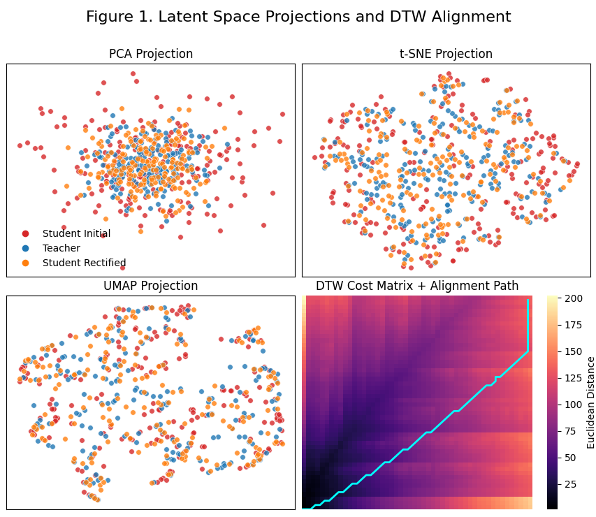
📍 Dimensionality Reduction and Related Methods
| Method | Category | Linear | Preserves | Mathematical Core | Typical Use Case |
|---|---|---|---|---|---|
| PCA | Dimensionality reduction | Yes | Global variance | Eigen-decomposition of covariance | Compression, noise reduction |
| t-SNE | Manifold learning | No | Local neighborhoods | KL divergence minimization | Visualization |
| UMAP | Manifold learning | No | Local + some global structure | Fuzzy simplicial sets | Visualization + clustering |
| DTW | Distance measure | No | Temporal alignment | Dynamic programming | Time-series similarity |
PCA (Principal Component Analysis)
-
The core idea of PCA is eigen-decomposition of the covariance matrix.
-
Covariance Matrix:
- Eigen-decomposition:
- Projection:
- where
t-SNE (t-Distributed Stochastic Neighbor Embedding)
-
The core idea of t-SNE is to minimize the KL divergence between probability distributions in the high-dimensional and low-dimensional spaces.
-
High-dimensional similarity (Gaussian):
- Low-dimensional similarity (Student t-distribution):
- Cost function:
UMAP (Uniform Manifold Approximation and Projection)
UMAP is based on fuzzy simplicial sets and optimized using cross-entropy.
- Fuzzy set membership:
- Symmetric membership:
- Low-dimensional edge weight:
- Binary cross-entropy objective:
DTW (Dynamic Time Warping)
-
DTW computes the minimum cumulative distance path between two sequences.
-
Distance matrix:
- Recursive accumulation:
- Boundary conditions:
\(D(0, 0) = 0\), \(D(0, \infty) = \infty\), \(D(\infty, 0) = \infty\)
Optimization and Scheduling
| Component | Configuration |
|---|---|
| Optimizer | AdamW (decoupled weight decay) |
| Weight Decay | 0.01 (applied to weight matrices only; excluded for bias and normalization parameters) |
| Learning Rate Scheduler | CosineAnnealingLR |
| Minimum Learning Rate | 1e-6 |
| Mixed Precision Training | Automatic Mixed Precision (fp16) with GradScaler |
| Gradient Clipping | Global norm clipping with max norm = 1.0 |
- The objects being regularized are: Linear weights of the Encoder, Non-linear mapping weights of the Projector
CE + KL define the task
Geo loss regularizes representation geometry
Weight decay regularizes parameter scale, not representation geometry

MLS dataset
Dataset: 59623 files x 4 epochs = 238,492 samples
Dev: 1248 transcripts, 1248 files
Initialization and State Management
| Component | Initialization |
|---|---|
| Teacher | Fully pretrained, encoder and decoder frozen |
| Student encoder | Pretrained Whisper-medium, frozen |
| Student decoder | Pretrained, frozen (with trainable LoRA adapters) |
| LoRA adapters | Randomly initialized (rank = 64), trainable |
| Projection module | Randomly initialized projection module |
| Optimizer state | Initialized from scratch if no checkpoint is loaded |
| Scheduler state | Fresh cosine learning rate schedule |
| AMP scaler | Initialized before training |
Core Generative Model Paradigms (Images / Video / Science)
| Model | Proposed by (Year) | Model Type | Core Idea (Essence) |
|---|---|---|---|
| Stable Diffusion | Stability AI et al. (2022) | Diffusion Model | Learn to reverse Gaussian noise step-by-step to generate images from text. |
| DALL·E | OpenAI (2021–2023) | Diffusion Model | Text-conditioned diffusion for image synthesis with strong semantic alignment. |
| OpenAI Sora | OpenAI (2024) | Diffusion + World Model | Diffusion in latent spacetime, learning physical and temporal consistency. |
| Meta MovieGen | Meta (2024) | Diffusion Model | High-fidelity video generation via large-scale diffusion with motion priors. |
| AlphaFold3 | DeepMind (2024) | Diffusion + Geometric Modeling | Diffusion over 3D molecular structures (proteins, DNA, ligands). |
| RFDiffusion | Baker Lab (2023) | Diffusion Model | Generate novel protein backbones via structure-space diffusion. |
Backpropagation
| Stage | Operation | Expression | Meaning |
|---|---|---|---|
| Forward Pass | Compute layer outputs | \(z^{(l)} = W^{(l)} a^{(l-1)} + b^{(l)}, \quad a^{(l)} = f(z^{(l)})\) | Obtain network predictions |
| Compute Loss | Compute error | \(L = \tfrac{1}{2}|\hat{y} - y|^2\) | Measure output error |
| Backward Pass | Backpropagate from output layer | \(\delta^{(L)} = (\hat{y} - y) \odot f'(z^{(L)})\) | Compute output-layer gradient |
| Propagate to previous layers | \(\delta^{(l)} = (W^{(l+1)})^T \delta^{(l+1)} \odot f'(z^{(l)})\) | Compute hidden-layer gradients | |
| Gradient Computation | Compute parameter gradients | \(\frac{\partial L}{\partial W^{(l)}} = \delta^{(l)} (a^{(l-1)})^T\) | Obtain weight gradients |
| Update | Update parameters | \(W^{(l)} \leftarrow W^{(l)} - \eta \frac{\partial L}{\partial W^{(l)}}\) | Optimize via gradient descent |
Optimal Method as Below with Hash Value
| Problem | Original Complexity | Optimal Complexity | Optimal Method | Further Optimization |
|---|---|---|---|---|
| Check Anagram | O(n) | O(n) | Counter / Hash Map | Cannot Be Improved |
| Dictionary Anagram Lookup | O(M × N log N) | O(M × N) | Hash Value + Character Count Key | Significantly Optimizable |
Hash Map and Graph for Optimization
| Analogy | Hash Map in Data Structures | Dynamic Programming / Graph in Algorithms |
|---|---|---|
| Essence | Trade space for time — achieve O(1) lookup. | Trade state-graph computation for optimal solution — typically O(N × M). |
| Advantage | Globally optimal method for key lookup. | Globally optimal framework for decision and optimization. |
| Limitation | Only applicable to key–value lookup problems. | Only applicable to decomposable problems with optimal substructure. |
| Conclusion | The most efficient in the lookup domain. | The most general but not universal in the optimization/decision domain. |
Languages
| Dimension | Rust | Go (Golang) | C++ | Python |
|---|---|---|---|---|
Essentially OOP | ✗ (OOP-like, but primarily functional) | ✗ (Has OOP features, but fundamentally procedural and concurrent) | ✓ (Classic, strongly object-oriented) | ✓ (Dynamic, fully object-oriented) |
| Programming Paradigm | Multi-paradigm: Primarily functional + systems, supports OOP traits | Procedural + concurrent, limited OOP | Multi-paradigm: Strongly object-oriented + generic | Multi-paradigm: Object-oriented + scripting |
| Type System | Static, compiled | Static, compiled | Static, compiled | Dynamic, interpreted |
| Memory Management | No GC; uses ownership + borrow checker | Automatic GC | Manual (new/delete) or smart pointers | Automatic GC |
| Concurrency Model | Lock-free, type-safe (“fearless concurrency”) | Goroutines + channels (CSP model) | Multithreading with manual locks | GIL limits true multithreading |
| Performance | Nearly equal to C++ | Close to C++, slightly slower (GC overhead) | Fastest native performance | Slowest (interpreted) |
| Safety | Compile-time memory safety; prevents data races | Memory-safe but not thread-safe | Very fast but error-prone (dangling pointers, overflows) | Safe but slow |
| Learning Curve | Steep (requires ownership understanding) | Easy (simple syntax) | Steep (complex syntax and templates) | Easiest (beginner-friendly) |
| Compile Speed | Slow | Fast | Slow (especially for large projects) | None (interpreted) |
| Ecosystem | Young but growing fast (systems, embedded, backend) | Mature (cloud, DevOps, microservices) | Broadest (systems, games, embedded) | Broadest (AI, data science, web) |
| Applications | System programming, secure backend, embedded, WebAssembly | Cloud-native systems, microservices, networking | OS, game engines, graphics | AI/ML, scripting, automation, data analysis |
| Philosophy | “Zero-cost abstraction” — safety + performance | “Pragmatic simplicity” — simplicity + efficiency | “Total control” — performance + flexibility | “Ease of use” — simplicity + rapid prototyping |
| Key Projects | Firefox, Tokio, AWS Firecracker | Docker, Kubernetes, Terraform | Unreal Engine, Chrome, TensorRT | PyTorch, TensorFlow, YouTube |
DNS
| IP Address | Service / Network | Description |
|---|---|---|
| 129.132.98.12 | ETH Zurich Primary DNS | Main campus DNS; default resolver used by EULER and VPN connections. |
| 129.132.250.2 | ETH Zurich Secondary DNS | Backup DNS paired with the primary resolver above. |
| 129.132.250.10 | SIS / Leonhard / LeoMed DNS | Internal DNS for Leonhard, LeoMed, and SIS Research IT environments. |
| 129.132.250.11 | SIS / Backup DNS | High-availability (HA) redundant DNS for research and secure clusters. |
Unix vs Linux - Concise Comparison
| Aspect | Unix (1969) | Linux (1991) |
|---|---|---|
| Creator | AT&T Bell Labs (Ken Thompson, Dennis Ritchie) | Linus Torvalds |
| Motivation | Replace the bloated Multics system with a simple, reliable operating system | Provide a free, Unix-compatible system that runs on inexpensive hardware |
| Cost | Expensive, proprietary | Free and open-source |
| License | Vendor-specific, closed-source | GNU GPL (open-source) |
| Status Today | Legacy and declining (e.g., Solaris, AIX, HP-UX) | Dominant platform (over 90% of servers, all top supercomputers) |
| Core Philosophy | Modularity: “Do one thing, and do it well” | Democratization of Unix through open collaboration |
Latent Space Structure
| Space | Core Definition | Difference from Others | Application Domains |
|---|---|---|---|
Hilbert Space | A complete inner product space where lengths, angles, and projections are well-defined | Serves as the foundational “perfect” geometric space; all others are generalizations or relaxations | Quantum mechanics, signal processing, optimization, machine learning |
| Banach Space | A complete normed vector space, not necessarily with an inner product | Has length but no angles | Non-Euclidean optimization, functional analysis |
| Riemannian Manifold | Each point has a local inner-product space (tangent space) | Locally Hilbert, globally curved | General relativity, geometric deep learning |
| Symplectic Space | Equipped with an area-preserving bilinear form | No distance, only conserved quantities | Classical mechanics, Hamiltonian systems |
| Topological Space | Defined only by neighborhood relationships, no metric required | No notion of length or angle | Generalized geometry, continuity, homotopy theory |
| Metric Space | A set with a defined distance function d(x, y) | Hilbert space is a special case | Clustering, manifold learning, distance-metric learning |
| Probability Space | A measurable space (Ω, F, P) defining random events | Describes the geometry of events | Probability theory, information geometry, Bayesian inference |
| Information Manifold | A Riemannian manifold on probability distributions | Uses Fisher information metric | Statistical inference, information geometry, variational inference |
| Kähler / Complex Space | Complex structure + symmetric geometry + metric | Conformal generalization of Hilbert space | Quantum geometry, string theory, complex optimization |
Algorithms
├── I. Data Structures
│   ├── Stack, Queue, <HashMap>, LinkedList
│
├── II. Algorithmic Patterns
│   ├── Two Pointers
│   ├── Sliding Window
│   ├── Prefix Sum
│   ├── Monotonic Stack / Queue
│   ├── Binary Search Patterns
│
├── III. Complex Algorithms
│   ├── <Dynamic Programming (DP)>
│   ├── <Graph Theory (DFS/BFS/Dijkstra)>
│   ├── Recursion / Backtracking
│   ├── Greedy Algorithms
│   ├── Divide & Conquer
│
└── IV. Problem Integration
    ├── Hard composite problems
    ├── Algorithm design questions
Diffusion, Stable Diffusion, Rectified Flow
| Dimension | Vanilla Diffusion Model (DDPM / DDIM) | Stable Diffusion (Latent Diffusion Model, LDM) | Rectified Flow (Flow Matching) |
|---|---|---|---|
| Start Distribution | Starts from pure Gaussian noise N(0, I) | Starts from latent-space noise (compressed through an encoder) | Starts from any distribution point (usually N(0, I), but customizable) |
| Generative Process | Multi-step denoising: reverses the noise diffusion process (xₜ₋₁ = fθ(xₜ, t)) | Multi-step denoising in latent space (computationally cheaper) (zₜ₋₁ = fθ(zₜ, t)) | Continuous one-step flow: learns an ODE (dxₜ/dt = vθ(xₜ, t)) |
| Mathematical Formulation | Discrete Markov chain (reverse SDE) | Discrete SDE in latent space | Continuous ODE or flow field |
| Computational Complexity | Multi-step sampling (20–1000 steps) | Multi-step but faster in latent space (20–50 steps) | Single continuous integration step |
| Advantages | High generation quality; theoretically grounded | High resolution, lightweight, and controllable (supports text prompts) | Fast convergence, continuous generation, minimal mode collapse |
| Limitations | Slow sampling; many denoising steps required | Strong dependence on encoder design and latent structure | Sensitive training stability; harder conditional control |
| Representative Papers / Applications | DDPM (Ho et al., 2020); DDIM (Song et al., 2021) | LDM / Stable Diffusion (Rombach et al., CVPR 2022) | Flow Matching / Rectified Flow (Liu et al., ICLR 2023) |
Optimization
| Component / Technique | Description | Implementation |
|---|---|---|
| Optimizer | Gradient-based weight updates with decoupled weight decay to improve stability on large models. | AdamW optimizer with lr=2.6e-4 and default β=(0.9, 0.999); stable for transformer-like models. |
| Learning-Rate Schedule | Smooth cosine decay to avoid abrupt gradient shocks after warm-up. | get_cosine_schedule_with_warmup(opt, 1000, 10000) — warm-up = 1 k steps, total = 10 k steps. |
| Warm-Up Phase | Gradually increases learning rate and KL weight to prevent early divergence in distillation. | Linear warm-up for both learning rate and λₖₗ (0 → 0.020584 during first 1000 steps). |
| Mixed-Precision Training | Uses half precision (torch.amp.autocast) to reduce GPU memory and improve throughput. | Forward/backward passes wrapped in autocast, scaled by GradScaler() for numerical stability. |
| Gradient Clipping | Prevents exploding gradients in long sequences. | torch.nn.utils.clip_grad_norm_(params, 1.0) each iteration. |
| Loss Function (Multi-Objective) | Balances semantic accuracy, distribution matching, and geometric alignment. | Total loss: L = LCE + λₖₗ · LKL + λGeo · LGeo, with λGeo = 0.969909 constant. |
| CE Loss | Supervised label alignment ensuring correct transcription semantics. | Cross-entropy between student predictions and true tokens. |
| KL Divergence | Soft-target distillation to transfer probability distributions from teacher logits. | F.kl_div(log_softmax(student/T), softmax(teacher/T)) · T², T = 2.0. |
| Riemannian Geodesic Loss | Aligns feature geometry on curved manifold instead of flat Euclidean MSE. | Geodesic distance = acos(cos_sim) between normalized hidden states. |
| Model Architecture (Student) | Lightweight CNN + Transformer hybrid for speech sequence modeling. | Two 1-D Conv layers → 6 Transformer encoder blocks → linear output head. |
| Teacher Model | Provides target logits and hidden features for distillation. | Frozen Whisper-large-v2 (FP16) encoder-decoder model. |
Structure
Machine Learning Fundamentals
      │
      ├── Data → Representation → Optimization → Generalization
      │       ├─ Focus: Data quality, bias mitigation, and representation learning
      │       ├─ Link to Gemini: multimodal data fusion (text, audio, vision, code)
      │       └─ Goal: Learn unified latent spaces that enable reasoning across modalities
      │
      ├── Deep Learning (CNN / RNN / Transformer)
      │       ├─ Forward & backward propagation as differentiable computation graphs
      │       ├─ Initialization, normalization, regularization → stability & convergence
      │       ├─ Loss design + learning rate scheduling → control of optimization dynamics
      │       └─ Transformer family as universal sequence learners (foundation for Gemini)
      │
      ├── Optimization & Geometry
      │       ├─ Gradient-based optimization viewed as navigating the loss landscape
      │       ├─ Flat vs. sharp minima → generalization and robustness trade-offs
      │       ├─ Riemannian geometry in embedding space → alignment on curved manifolds
      │       └─ Connection: Gemini’s embedding consistency and representation curvature
      │
      ├── Model Compression & Distillation
      │       ├─ Knowledge transfer from large to small models (teacher → student)
      │       ├─ Soft vs. hard labels → probabilistic vs. symbolic supervision
      │       ├─ LoRA / Adapter-based fine-tuning → parameter-efficient adaptation
      │       ├─ Trade-offs: accuracy ↔ latency ↔ memory footprint ↔ energy efficiency
      │       └─ Relevance: LearnLM and Gemini use adapter-tuned submodels for learning tasks
      │
      └── ML Engineering & Responsible AI
              ├─ Data pipelines, reproducibility, evaluation, and continuous integration
              ├─ Monitoring, checkpointing, scalable deployment on distributed accelerators
              ├─ Safety alignment and interpretability — understanding model decisions
              ├─ Evaluation beyond accuracy: robustness, fairness, value alignment
              └─ Ethical ML engineering: accountability and transparency in large systems
Time
| Big-O | Name | Typical Example |
|---|---|---|
| O(1) | Constant time | Accessing array element |
| O(log n) | Logarithmic time | Binary search |
| O(n) | Linear time | Single loop through array |
| O(n log n) | Linearithmic time | Merge sort, Quick sort |
| O(n²) | Quadratic time | Nested loops, Bubble sort |
| O(n³) | Cubic time | Triple nested loops |
| O(2ⁿ) | Exponential time | Subset / permutation generation |
| O(n!) | Factorial time | Traveling Salesman, N-Queens |
| O(bᵈ) | Branching search | DFS in state tree with branching b and depth d |
O(n):            O(n log n):                 O(n²):
loop → → →       divide → sort → merge      double loop → compare all
(one pass)       (log layers × n work)       (each pair compared)
linear scan       merge / quick sort         bubble / selection sort
Space
| Big-O | Name | Typical Example |
|---|---|---|
| O(1) | Constant space | In-place swap, variable assignment |
| O(log n) | Logarithmic space | Recursive binary search |
| O(n) | Linear space | Storing array, dynamic programming 1-D |
| O(n²) | Quadratic space | 2-D matrix, Floyd-Warshall DP |
| O(n³) | Cubic space | 3-D DP table |
| O(2ⁿ) | Exponential space | Memoization of all subsets |
Protocol and Ports
[You: MacBook]  ←→  [Encrypted Tunnel (AES)]  ←→  [Mac Studio Server]
         ↕                             ↕
   ssh user@ip_address         sshd (daemon listening on port 22)
| Protocol | Port | Purpose |
|---|---|---|
| HTTP | 80 | Web traffic |
| HTTPS | 443 | Secure web traffic |
| FTP | 21 | File transfer |
| SSH | 22 | Secure remote shell |
| Function | Command Example | Description |
|---|---|---|
Remote Login | ssh user@192.xxx.x.xx | Open a command-line session on a remote computer |
File Transfer | scp file.txt user@host:/path/ | Securely copy a file to a remote machine |
Port Forwarding | ssh -L 8080:localhost:80 user@host | Map a remote port to a local port through an encrypted tunnel |
| Passwordless Login | Public key authentication (~/.ssh/id_rsa.pub) | Automatically authenticate using key pairs |
| Automation Control | Use SSH to execute commands or sync data in bulk | Common in DevOps or HPC environments |
REST API
| Endpoint | Method | Description | Parameters | Response | Status Codes |
|---|---|---|---|---|---|
| /users | GET | Get all users | none | list of users | 200 OK |
| /users | POST | Create a new user | username:string, password:string | created user | 201 Created |
| /users/{id} | GET | Get user by ID | id:int | user object | 200 OK / 404 Not Found |
| /users/{id} | PUT | Update user | username:string | updated user | 200 OK |
| /users/{id} | DELETE | Delete user | id:int | none | 204 No Content |
AI API
| Endpoint | Method | Description | Parameters | Response | Status |
|---|---|---|---|---|---|
| /ai/chat | POST | Generate AI response | message:string | AI text | 200 |
| /ai/image | POST | Generate image | prompt:string | image URL | 200 |
Structure
Frontend
   ↓
Controller (REST API)
   ↓
DTO
   ↓
Mapper
   ↓
Entity
   ↓
Repository
   ↓
Database
| Concept | Essence | Purpose |
|---|---|---|
| REST API | Communication interface | Enables clients to interact with the server through HTTP requests |
| DTO (Data Transfer Object) | Data structure | Defines the format of data exchanged between client and server |
| Mapper | Conversion utility | Converts data between DTOs and Entities |
Optimizers
| Era | Optimizer | Year | Core Innovation | Key Equation / Concept | Limitation Solved | Remarks |
|---|---|---|---|---|---|---|
| Classical GD | Gradient Descent (GD) | 1951 | Update weights along the negative gradient direction | \(w_{t+1} = w_t - \eta \nabla L(w_t)\) | None (too simple) | Foundation of all optimizers |
| Stochastic Gradient Descent (SGD) | 1983 | Uses random mini-batches to improve efficiency | \(\nabla L(w_t) \approx \frac{1}{\lvert B \rvert} \sum_{i \in B} \nabla L_i(w_t)\) | High variance and slow convergence | Enables online / large-scale learning | |
| Momentum Era | SGD + Momentum | 1989 | Adds velocity term to accumulate past gradients | \(v_t = \beta v_{t-1} + (1-\beta)\nabla L(w_t), \quad w_{t+1} = w_t - \eta v_t\) | Oscillations in narrow valleys | Faster convergence, physics-inspired |
| Nesterov Accelerated Gradient (NAG) | 1991 | Looks ahead using gradient of estimated future position | \(v_t = \beta v_{t-1} + (1-\beta)\nabla L(w_t - \eta \beta v_{t-1})\) | Overshooting in Momentum | Smoother convergence and stability | |
| Adaptive Learning | Adagrad | 2011 | Per-parameter adaptive learning rate | \(G_t = \sum_{\tau=1}^{t} g_\tau^2, \quad \eta_{t,i} = \frac{\eta}{\sqrt{G_{t,i}}+\epsilon}\) | Manual learning rate tuning | Excellent for sparse features (NLP) |
| RMSProp | 2012 | Exponentially weighted moving average of squared gradients | \(v_t = \rho v_{t-1} + (1-\rho)g_t^2, \quad w_{t+1} = w_t - \frac{\eta}{\sqrt{v_t+\epsilon}}g_t\) | Adagrad’s decaying rate problem | Stable for non-stationary objectives | |
| Modern Standard | Adam | 2014 | Combines Momentum and RMSProp | \(m_t = \beta_1 m_{t-1} + (1-\beta_1)g_t, \quad v_t = \beta_2 v_{t-1} + (1-\beta_2)g_t^2\) \(\hat{m}_t = \frac{m_t}{1-\beta_1^t}, \quad \hat{v}_t = \frac{v_t}{1-\beta_2^t}, \quad w_{t+1} = w_t - \eta \frac{\hat{m}_t}{\sqrt{\hat{v}_t}+\epsilon}\) | Gradient noise and curvature imbalance | Default optimizer for most deep networks |
| AdamW | 2017 | Decouples weight decay from gradient update | \(w_{t+1} = w_t(1-\eta\lambda) - \eta \frac{m_t}{\sqrt{v_t}+\epsilon}\) | L2 regularization bias in Adam | Default for Transformer / LLM training | |
| Geometry-Aware & Large Batch | LARS (Layer-wise Adaptive Rate Scaling) | 2018 | Layer-wise adaptive learning rate | \(\eta_l = \eta \frac{|w_l|}{|g_l|+\epsilon}\) | Scale mismatch in large-batch training | Used in ResNet / ImageNet large-batch setups |
| LAMB (Layer-wise Adaptive Moments) | 2019 | Extends LARS with Adam-style moments | \(r_t = \frac{|w_t|}{|\hat{m}_t / (\sqrt{\hat{v}_t}+\epsilon)|}, \quad w_{t+1}=w_t - \eta r_t \frac{\hat{m}_t}{\sqrt{\hat{v}_t}+\epsilon}\) | Poor scaling of Adam for huge batches | Core optimizer for BERT, GPT | |
| Variance Rectification & Belief Models | RAdam | 2019 | Rectifies variance of adaptive learning rate | \(\eta_t = \eta \frac{\sqrt{(1-\beta_2^t)/(1-\beta_2)}}{\sqrt{v_t}+\epsilon}\) | Instability in early training | More robust warm-up-free Adam |
| AdaBelief | 2020 | Tracks belief in gradient direction | \(v_t = \beta_2 v_{t-1} + (1-\beta_2)(g_t - m_t)^2\) | Gradient over-smoothing | Better generalization for small datasets | |
| Second-Order & Natural Gradient | K-FAC (Kronecker-Factored Approximate Curvature) | 2015–2023 | Approximates curvature via blockwise Kronecker products | \(F^{-1} \approx A^{-1} \otimes B^{-1}, \quad w_{t+1} = w_t - \eta F^{-1}\nabla L\) | Ignores curvature in SGD/Adam | Faster convergence, heavy memory use |
| Shampoo | 2021 | Matrix preconditioning per layer | \(G_t = \sum_{\tau=1}^{t} g_\tau g_\tau^\top, \quad W_{t+1}=W_t - \eta G_t^{-1/2}\nabla L\) | Slow convergence on ill-conditioned loss | Improves conditioning for large models | |
| Modern LLM Optimizers | Lion | 2023 | Momentum with sign-based updates | \(w_{t+1} = w_t - \eta \, \text{sign}(\beta_1 m_t + (1-\beta_1)g_t)\) | Over-adaptation of Adam | Efficient and strong generalization for LLMs |
| Sophia | 2023 | Second-order curvature-aware optimizer | \(w_{t+1} = w_t - \eta \frac{g_t}{\sqrt{h_t+\epsilon}}, \quad h_t \approx \text{diag}(H_t)\) | Slow convergence in large-scale Adam | State-of-the-art for Transformer training |
TAID
Initial training (step=0): λ=0.1 intermediate = 0.9 * student_probs + 0.1 * teacher_probs
→ Mainly learn the student’s own distribution
Mid-training (step=400): λ≈0.5 intermediate = 0.5 * student_probs + 0.5 * teacher_probs
→ Balanced learning
Late training (step=800): λ=0.9 intermediate = 0.1 * student_probs + 0.9 * teacher_probs
→ Mainly learn the teacher’s distribution
Background Knowledge
RL On Diffusion
I. Base Diffusion Backbone (Generative Prior)
Input (x₀ = real data sample: image, trajectory, audio, 3D scene)
      ↓
Forward Diffusion Process (adds Gaussian noise)
      ↓
x₁ ← √α₁·x₀ + √(1−α₁)·ε₁
x₂ ← √α₂·x₁ + √(1−α₂)·ε₂
⋮
x_T ≈ pure Gaussian noise N(0, I)
      ↓
Reverse Denoising Process (parameterized by neural network ε_θ)
      ↓
x_{t−1} = (x_t − √(1−α_t)·ε_θ(x_t, t, cond)) / √α_t + η·σ_t
      ↓
UNet / Transformer backbone → learns to reconstruct x₀
II. Policy Representation via Diffusion
Environment State s_t
      ↓
Noise z_t ~ N(0, I)
      ↓
Diffusion Policy Network ε_θ(s_t, z_t, t)
      ↓
Sample Action a_t = Denoise(z_t | s_t)
      ↓
Execute Action in Environment → Receive Reward r_t
      ↓
Collect Trajectory τ = {s_t, a_t, r_t}
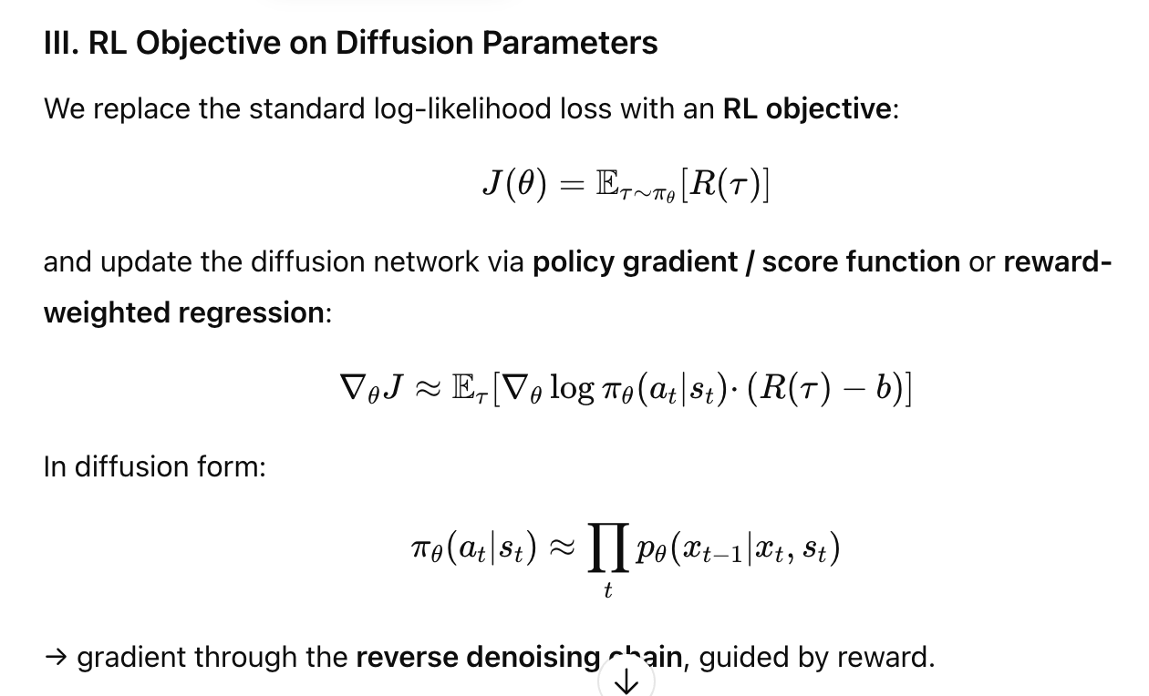
IV. Reward-Guided Diffusion Training (Diffusion Policy Optimization)
For each episode:
  1. Sample noise x_T ~ N(0, I)
  2. Run reverse diffusion (ε_θ) conditioned on state s_t
  3. Generate predicted action trajectory x₀
  4. Execute in environment → collect reward R
  5. Compute loss:
         L_total = L_diffusion + λ·L_RL
         L_RL = − E[R(τ)]
  6. Backpropagate through ε_θ network
Diffusion Policy, Decision Diffuser
Random Noise in Action Space
      ↓
Diffusion or Flow Process
      ↓
Denoising Steps / Continuous Flow
      ↓
Policy Network predicts εθ(x_t,t)
      ↓
Clean Action Sequence (Optimal Trajectory)
      ↓
Execute in Environment (Robotics / Control)
| Function | Formula | Derivative | Core Idea | Usage / Notes |
|---|---|---|---|---|
| Sigmoid | \(f(x) = \frac{1}{1 + e^{-x}}\) | \(f'(x) = f(x)\,[1 - f(x)]\) | Smooth bounded mapping (0, 1) | Common in probabilistic outputs |
| Tanh | \(f(x) = \tanh(x) = \frac{e^x - e^{-x}}{e^x + e^{-x}}\) | \(f'(x) = 1 - f(x)^2\) | Zero-centered output | Improves symmetry over Sigmoid |
| ReLU | \(f(x) = \max(0,\,x)\) | \(f'(x)=\begin{cases}1,&x>0\\0,&x\le0\end{cases}\) | Sparse and efficient | Fast convergence, stable training |
| Leaky ReLU | \(f(x)=\max(\alpha x,\,x)\) | piecewise constant | Avoids dead neurons | Small negative slope for x < 0 |
| Swish / SiLU | \(f(x)=x\,\sigma(x),\ \sigma(x)=\frac{1}{1+e^{-x}}\) | \(f'(x)=\sigma(x)+x\,\sigma(x)[1-\sigma(x)]\) | Smooth, self-gated ReLU | Used in Google EfficientNet |
| Mish | \(f(x)=x\,\tanh(\ln(1+e^x))\) | smooth | Non-monotonic, better gradient flow | Used in YOLOv4, ResNet variants |
| GELU | \(f(x)=x\,\Phi(x),\ \Phi(x)\text{: Gaussian CDF}\) | smooth | Probabilistic gating | Default in Transformers (BERT, GPT) |
| JumpReLU (DeepMind) | \(f(x)=\max(0,\,x-j),\ j\text{ learned}\) | piecewise constant | Learnable sparsity threshold | Used in Sparse Autoencoders for interpretability |
| Softmax | \(f_i(x)=\frac{e^{x_i}}{\sum_j e^{x_j}}\) | — | Converts logits → probabilities | Standard output for classification |
Learning Rates
| Trend | Description | Representative Systems |
|---|---|---|
| Cosine + Warmup → Standard Default | Most stable across architectures. | ViT, GPT-J, Whisper, Stable Diffusion |
| Adaptive + Restart Hybrids | Combine SGDR + ReduceLROnPlateau. | DeepSpeed, Megatron-LM, PaLM 2 |
| Optimizer-Integrated Scheduling | Scheduler coupled with optimizer (AdamW, LAMB). | GPT-4, Gemini 1.5, Claude 3 |
| Noisy / Stochastic Schedules | Inject noise to encourage flat minima. | Google Brain NAS, RL-based training |
| Dynamic Data-Aware LR Control | LR adapted by validation loss or gradient norm. | Reinforcement fine-tuning (RLHF, PPO) |
Scaling Law
| Year | Model | Number of Layers | Parameter Count | FLOPs (per inference) | Activations (per forward pass) | Typical Memory Footprint |
|---|---|---|---|---|---|---|
| 1998 | LeNet | 5 | ~0.1 M | ~0.001 GFLOPs | < 1 MB | < 10 MB |
| 2012 | AlexNet | 8 | 60 M | ~1.5 GFLOPs | ~100 MB | ~1 GB |
| 2015 | VGG-16 | 16 | 138 M | ~15 GFLOPs | ~200 MB | ~2–4 GB |
| 2016 | ResNet-152 | 152 | 60 M | ~11 GFLOPs | ~250 MB | ~4–6 GB |
| 2018 | BERT-Large | 24 | 340 M | ~180 GFLOPs | ~1 GB | ~10–12 GB |
| 2020 | GPT-3 | 96 | 175 B | ~3.1 × 10¹² FLOPs | ~20 GB | ~350 GB (weights) / > 1 TB (training) |
| 2024 | GPT-4 / Gemini 1.5 / Claude 3 | ~120 – 200 | > 1 T (trillion) | ~10¹³ – 10¹⁴ FLOPs | > 50 GB (activations) | Multiple TB (large-scale training) |
Generalization and Regularization
Underfitting:     Overfitting:        Good Embedding:
 • • • • •        ●●●  ○○○  ▲▲▲       ● ●   ○ ○   ▲ ▲
 ○ ○ ○ ○ ○        (tight) (tight)      (clear but smooth)
 ▲ ▲ ▲ ▲ ▲        val points outside   val & train overlap
| Principle | Intuition |
|---|---|
| Regularization = adding controlled noise or constraints to prevent memorization. | Introduces noise or limits (e.g., dropout, weight decay, data augmentation) so the model learns general patterns instead of memorizing the training set. |
| Overfitting = perfect fit on training data, poor generalization. | The model minimizes training loss too well, capturing noise instead of true structure — leads to poor performance on unseen data. |
| Goal = flatter minima + smoother decision boundaries. | Seek regions in the loss landscape where small parameter changes do not greatly affect loss — resulting in more stable, generalizable models. |
Forward Pass
Input (32×32×3)
      ↓
Conv (3×3 kernel, 16 filters)
      ↓
ReLU activation
      ↓
Max Pooling (2×2)
      ↓
Conv (3×3 kernel, 32 filters)
      ↓
ReLU
      ↓
Global Avg Pooling
      ↓
Flatten → Dense (Fully-connected)
      ↓
Softmax → [Cat, Dog, Car, …]
Optimizations for Training
| Stage | Method | Purpose / Effect |
|---|---|---|
| Initialization Stage | Xavier / He initialization | Avoid falling into poor regions at the start |
| Early Exploration Stage | Large learning rate + Momentum | Maintain global exploration ability |
| Mid Convergence Stage | Adam / RMSProp + Cosine Annealing | Ensure smooth descent and curvature adaptation |
| Late Fine-tuning Stage | SAM / Entropy-SGD / Weight Decay | Locate flat minima and enhance generalization |
| During Training | Mini-batch noise + Dropout | Prevent getting stuck at saddle points |
| Architectural Level | Residual connections / Normalization layers | Improve gradient flow and smooth the optimization landscape |
Normalization and Regularization in different Model Structures
| Item | L1 Regularization | L2 Regularization |
|---|---|---|
| Shape | Diamond-shaped constraint | Circular constraint |
| Optimum Point | Usually lies on the coordinate axes (sparse solution) | Usually lies on the circle (continuous shrinkage) |
| Result | Some weights are “cut” to exactly 0 | All weights are smoothly reduced but remain non-zero |

| Model Example | Normalization | Regularization | Essence & How It Works |
|---|---|---|---|
| CNN (e.g., ResNet) | Batch Normalization — normalizes activations within a mini-batch to stabilize gradients and speed up convergence. | Weight Decay + Dropout — penalizes large weights and randomly drops neurons to reduce overfitting. | Normalization equalizes feature scales during training, while Regularization constrains model capacity to improve generalization. |
| Transformer / LLM | Layer Normalization — normalizes hidden states across features to maintain stable activations in deep attention layers. | Attention Dropout + L2 Regularization — randomly masks attention links and adds weight penalties to prevent overfitting. | Normalization stabilizes internal representations; regularization prevents memorization of training data. |
| MLP | Input Standardization — rescales each input feature to zero mean and unit variance. | L2 Regularization (Ridge) — discourages large parameter magnitudes for smoother mappings. | Normalization improves numerical stability; regularization enforces simpler models with better generalization. |
Optimized Decoding
Classical Decoding (Without KV Cache)             Optimized Decoding (With KV Cache)

 ┌───────────────┐                                ┌────────────────────────┐
 │   Decoder     │                                │   Decoder + KV Cache   │
 │  (Self-Attn)  │                                │  (Self-Attn + Storage) │
 └───────┬───────┘                                └──────────┬─────────────┘
         │                                                   │
         ▼                                                   ▼
 ┌───────────────┐                                ┌─────────────────────────┐
 │ Recompute all │   O(n²) per step               │  Reuse stored K/V       │
 │ past tokens   │ -----------------------------> │  Only new Q calculated  │
 │ at every step │                                │  O(n) per step          │
 └───────────────┘                                └─────────────────────────┘
         │                                                     │
         ▼                                                     ▼
     ┌─────────┐                                       ┌───────────────┐
     │ Latency │                                       │  Low Latency  │
     │  High   │                                       │  On-Device OK │
     └─────────┘                                       └───────────────┘

   - Redundant computation                           - No recomputation
   - High memory bandwidth                           - Lower memory & power
   - Slow inference                                  - Faster inference
Transformer Assembly Line
═══════════════════════════════════════════════════════
Raw Donuts → Community Check → Solo Decoration → Finished Donuts
(Input)       (Attention)       (FFN)            (Output)
    ↓             ↓                ↓               ↓
┌─────────┐  ┌──────────────┐  ┌──────────────┐    ┌─────────┐
│ Plain   │→ │  Community   │→ │   Solo       │ →  │Gourmet  │
│ Donuts  │  │  Analysis    │  │ Decoration   │    │Donuts   │
└─────────┘  └──────────────┘  └──────────────┘    └─────────┘
   ↓                ↓                 ↓                 ↓
   X₀          X₁ = Attention     X₂ = FFN            Output

 1. X₁ᵢ = Σⱼ αᵢⱼ × V_j               (Global Linear)
 2. X₂ᵢ = W₂·ReLU(W₁·X₁ᵢ + b₁) + b₂  (Local Nonlinear)

Attention: Convex combination → Stays within input space
FFN: Nonlinear transformation → Can transcend input space
Activation Function Characteristics Comparison
═════════════════════════════════════════════════
┌──────────┬────────────┬───────────────┬──────────────┬─────────────┐
│Function  │ Smoothness │ Computational │ Gradient     │ Performance │
│          │            │ Complexity    │ Properties   │             │
├──────────┼────────────┼───────────────┼──────────────┼─────────────┤
│ ReLU     │ Non-smooth │ Minimal       │ Sparse       │ Baseline    │
│ GELU     │ Smooth     │ Moderate      │ Dense        │ Better      │
│ SwiGLU   │ Smooth     │ High          │ Gated        │ Best        │
│ Mish     │ Very Smooth│ High          │ Adaptive     │ Very Good   │
│ Swish    │ Smooth     │ Moderate      │ Self-gated   │ Good        │
│ ELU      │ Smooth     │ Moderate      │ Negative-safe│ Good        │
└──────────┴────────────┴───────────────┴──────────────┴─────────────┘
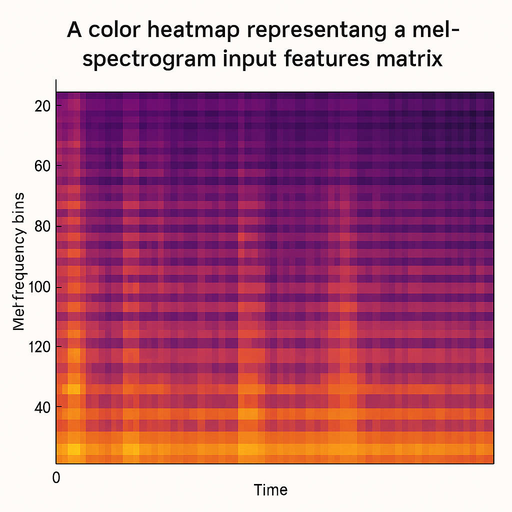
Input Features From Whisper
Why T≈499
- Whisper feature extractor
- The original audio (30 s) generates about 3000 frames of 80-dimensional log-Mel features at a granularity of 10 ms per frame
- Whisper first divides the original mono audio (30 seconds, 16 kHz) into several short segments
- Generate an 80-dimensional log-Mel feature every 10 ms
- 30 s / 0.01 s = 3000 frames
- These 3000 frames are still very dense. If Transformer processes them directly, the computational workload and memory requirements will be too high
- Before being fed into the Transformer encoder, these 3000 frames are first downsampled through a convolutional layer (stride=2), and then continuously merged or downsampled in the multi-layer Transformer block
- The final output length is about 3000 / 2 / 3 = 500 frames (actually 499 frames)
30 s audio
    ⇓ (extract 80-dim log-Mel every 10 ms)
3000 frames
    ⇓ (convolutional layer with stride=2)
1500 frames
    ⇓ (further down-sampling/merging inside the Transformer encoder ≈×3)
    ⇓ (Pooling or Conv1d: kernel_size=3, stride=3)
≈500 frames  (actually 499 frames)
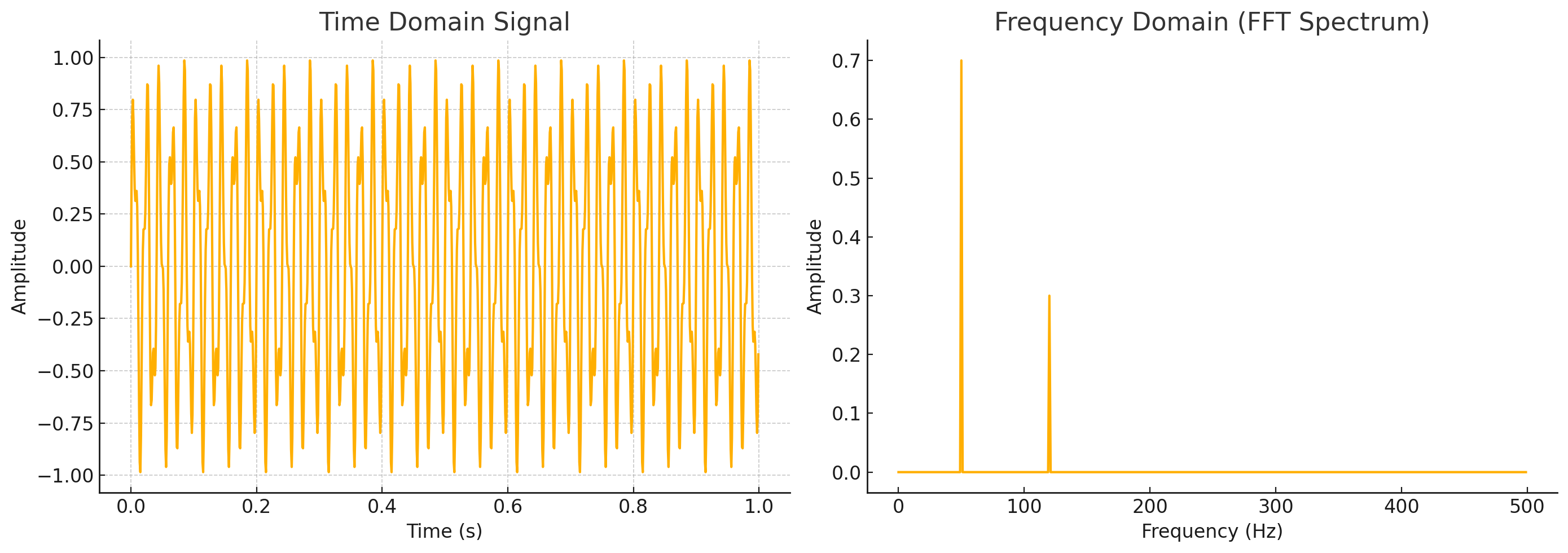
Audio Signal Characteristics - Redundancy -> why can be compressed to T~499 frames
1. Audio frame rate is typically high
sample_rate = 16000      # 16 kHz sampling rate
frame_rate = 100         # 100 frames per second
frame_duration = 10      # 10 ms per frame

2. 30 seconds of audio
total_frames = 30 * frame_rate  # 3000 frames

3. Adjacent frames are highly correlated
correlation_coefficient ≈ 0.9  # typical inter-frame correlation
Orignial LoRA Paper
ΔW = A · B -> only low-rank increments are made to W_q and W_v in the attention
Choices of LoRA Injection
decoder.layers.*.encoder_attn.q_proj
decoder.layers.*.encoder_attn.v_proj
decoder.layers.*.self_attn.q_proj
decoder.layers.*.self_attn.v_proj
Temperature
- Initial pilot temperature:
T = - Search range:
[ ] - Optuna hyperparameter: include
tempas a tunable parameter - Guidance: prevent over-smoothing (i.e. avoid
T > 5)
Hard vs. Soft Labels in Knowledge Distillation
-
Hard Labels: one-hot vectors from ground truth
y = [0, …, 1, …, 0]
• Strong supervision → binary certainty
• Forces correct classification -
Soft Labels: teacher’s softmax outputs
p_teacher = [0.6, 0.3, 0.1]
• Confidence & uncertainty
• Encodes inter-class similarity
Why num_workers Affects GPU Performance
The num_workers parameter in PyTorch DataLoader controls the number of CPU processes responsible for data loading and preprocessing. This directly impacts GPU utilization through data pipeline optimization
Performance Comparison
Single-threaded (num_workers=0)
- CPU: Load→Preprocess→Transfer, GPU idle, Load→Preprocess→Transfer
- GPU: Idle, Compute, Idle
Multi-threaded (num_workers=4)
- CPU: Continuous data preparation (4 parallel threads)
- GPU: Continuous computation (minimal idle time)
Key Insight
- Increasing num_workers enhances “CUDA kernel parallelism” not by adding GPU parallelism, but by eliminating GPU starvation. Multiple CPU workers ensure the GPU receives a steady stream of preprocessed data, maximizing hardware utilization and reducing training time
- The optimal num_workers typically ranges from 2-4 per GPU, depending on CPU core count and I/O bottlenecks
CTC Loss - Hard Supervision - Here Cross-Entropy (CE) Loss since Whisper is Seq2Seq with Decoders
Since Whisper is a Seq2Seq model with Decoder, cross-entropy loss is employed here.
The decoder generates hidden state sequences at step $u$: \(\{\mathbf{d}_u\}_{u=1}^U\)
mapping to the target text sequence: \(\{y_u\}_{u=1}^U\)
using token-by-token one-to-one supervision:
- Token-to-Token Alignment Each step has a clear “correct” next token, requiring no implicit alignment
- One-Step Supervision Cross-entropy is directly applied to the prediction distribution at each position $u$
- Direct Gradient Backpropagated from the output layer, enabling stable convergence
Cross-Entropy Loss Formula \(\mathcal{L}_{\mathrm{CE}} = -\sum_{u=1}^U \log P_\theta\bigl(y_u \mid y_{<u}, \mathbf{h}_{1:T}\bigr)\)
where:
- $\mathbf{h}_{1:T}$ represents the audio representation output by the encoder
- $y_{<u}=(y_1,\dots,y_{u-1})$ are the previously generated tokens
- $U$ is the target sequence length
Following the encoder’s output audio frame sequence: \(\{\mathbf{h}_t\}_{t=1}^T\)
mapping to transcript tokens: \(\{y_u\}_{u=1}^U\)
without explicit frame-level labels:
- Frame-to-Token Alignment Automatic alignment from audio frames to text tokens
- Marginalizing Paths Marginalizing over all possible alignment paths
- Gradient Signal Gradient signals propagate to all relevant audio frames through attention mechanisms
Hyperparameter Optimization
Knowledge fidelity × Geometric alignment × Optimization stability
def objective(trial):
    lambda_kl  = trial.suggest_loguniform("lambda_kl", 1e-2, 1e1)
    lambda_geo = trial.suggest_loguniform("lambda_geo", 1e-3, 1e0)
    lr         = trial.suggest_loguniform("lr", 5e-5, 5e-4)

    wer = train_and_evaluate(
        lambda_kl=lambda_kl,
        lambda_geo=lambda_geo,
        learning_rate=lr
    )
    return wer
Background Knowledge 2
[Training Neural Network]
      │
      ▼
[Problem: Overfitting]
      │  model performs well on train set
      └─ poor generalization on unseen data
      ▼
[Regularization Strategies]
      │
      ├─ L1 Regularization → add |w| penalty
      │     encourages sparsity, feature selection
      │
      ├─ L2 Regularization (Weight Decay)
      │     adds w² penalty, smooths weights
      │     reduces variance, stabilizes gradients
      │
      ├─ Early Stopping
      │     monitor validation loss → stop early
      │
      ├─ Data Augmentation
      │     enlarge dataset (flip, crop, color jitter)
      │     improves robustness & invariance
      │
      └─ Dropout
            randomly deactivate neurons (mask m)
            prevents co-adaptation
            during inference: scale activations by p
      ▼
[Normalization Layers]
      │
      ├─ Batch Normalization (BN)
      │     normalize activations per mini-batch
      │     μ_B, σ_B computed over batch samples
      │     then apply γ (scale) + β (shift)
      │     allows larger learning rate & faster training
      │
      ├─ Layer Normalization (LN)
      │     normalize across features, not batch
      │     used in Transformers (batch-size independent)
      │
      └─ Effect:
            stabilizes gradient flow
            reduces internal covariate shift
            improves convergence speed
      ▼
[Residual Connections]
      │
      └─ skip connection y = F(x) + x
            eases gradient propagation
            enables very deep CNNs (ResNet)
      ▼
[Combined Strategy]
      │
      ├─ Regularization (L1/L2)
      ├─ Dropout
      ├─ Batch Normalization
      └─ Data Augmentation
      ▼
[Result]
      │
      └─ High generalization, stable training,
         smoother optimization landscape,
         reduced overfitting risk
[Closed-Set Classification]
      │
      └─ assumes all test classes are known
         model outputs one of O fixed labels
      ▼
[Open-Set Problem]
      │
      ├─ real-world contains unknown categories
      ├─ standard SoftMax → overconfident wrong predictions
      └─ need to reject unseen (unknown) samples
      ▼
[Goal: Open-Set Recognition]
      │
      ├─ recognize known classes correctly
      └─ detect / reject unknown classes (OOD)
      ▼
[Two Main Paradigms]
      │
      ├─ Two-Stage OSR
      │     Stage 1: detect unknowns (OOD)
      │     Stage 2: classify known samples
      │
      └─ Integrated OSR
            single model learns known + reject class
            adds “unknown” logits or rejection threshold
      ▼
[Core Approaches]
      │
      ├─ OSDN (Open-Set Deep Network)
      │     compute Mean Activation Vector (MAV)
      │     distance D_o = ||ϕ - μ_o||
      │     fit EVT (Extreme Value Theory) model to tails
      │
      ├─ GHOST (Gaussian Hypothesis OSR)
      │     per-class Gaussian modeling in feature space
      │     normalize logits by (μ_o, σ_o)
      │     provides calibrated confidence
      │
      ├─ Garbage / Background Class
      │     add class y₀ for “none of the above”
      │     weighted loss: λ_τ = N / ((O+1)N_τ)
      │
      ├─ Entropic Open-Set Loss
      │     for unknowns, enforce uniform SoftMax
      │     target: t_o = 1/O for all o
      │     equalizes logits → high entropy
      │
      └─ Confidence Thresholding
            use ζ threshold on SoftMax
            accept if max(ŷ_o) > ζ, else reject
      ▼
[Training]
      │
      ├─ Known samples: one-hot targets
      ├─ Unknown samples: uniform targets
      └─ Loss combines CE + Entropic term
      ▼
[Evaluation Metrics]
      │
      ├─ CCR (Correct Classification Rate)
      │     true positives among known samples
      │
      ├─ FPR (False Positive Rate)
      │     unknowns misclassified as knowns
      │
      └─ OSCR Curve (CCR vs FPR)
            area under curve (AUOSCR) = performance
      ▼
[Modern Implementations]
      │
      ├─ ImageNet-based OSR protocols (P1–P3)
      ├─ Feature-space Gaussian models (GHOST)
      ├─ Entropic loss + background class hybrid
      └─ Evaluation by AIML UZH / WACV 2023
      ▼
[Outcome]
      │
      └─ OSR enables reliable recognition under uncertainty:
         “I know what I know — and I know what I don’t.”
ResNet
Plain Net:                 ResNet:

Input                      Input
  │                          │
[Conv]                    [Conv]
  │                          │
[Conv]        vs         [Conv] +───┐
  │                          │      │
[Conv]                    [Conv] ◄──┘
  │                          │
Output                     Output

# Pooling Layer
Local region
┌───────────────┐
│   weak   weak │
│               │
│   weak  STRONG│  ──►  STRONG
└───────────────┘

# 2D + 3D Convolution
Input: H × W × C
Kernel: k × k × C

Input: H × W × T × C
Kernel: k × k × k × C
| Stage | Process | Mathematical Meaning | Intuitive Explanation |
|---|---|---|---|
| Forward Process | Add Gaussian noise to clean trajectories \((x_0 \rightarrow x_T)\). | \(q(x_t \mid x_{t-1}) = \mathcal{N}(\sqrt{1 - \beta_t} \, x_{t-1}, \, \beta_t I)\) | Gradually “scrambles” a human driving path — this step is fixed and not learned. |
| Reverse Process | Learn to denoise noisy trajectories \((x_T \rightarrow x_0)\) conditioned on perception \(c\). | \(p_\theta(x_{t-1} \mid x_t, c) = \mathcal{N}(\mu_\theta(x_t, t, c), \Sigma_\theta)\) | The model learns to “restore order from noise,” reconstructing human-like trajectories that fit the scene. |
| Prior-Guided Learning | Add an Anchored Gaussian prior for realistic initialization. | \(x_T \sim \mathcal{N}(\mu_{anchor}, \sigma^2 I)\) | The model doesn’t predict trajectories directly—it learns to move toward the probability distribution of human driving behaviors. |
Temporal Alignment Leakage
┌─────────────────────────────────────────┐
│  Temporal Downsampling Effect           │
│                                         │
│  Teacher Sequence (1500 frames)         │
│  ┌─┬─┬─┬─┬─┬─┬─┬─┬─┬─┬─┬─┬─┬─┬─┬─┬─┬─┐  │
│  │▓│▓│▓│▓│▓│▓│▓│▓│▓│▓│▓│▓│▓│▓│▓│▓│▓│▓│  │
│  └─┴─┴─┴─┴─┴─┴─┴─┴─┴─┴─┴─┴─┴─┴─┴─┴─┴─┘  │
│          ↓ 3:1 compression              │
│  Student Sequence (499 frames)          │
│  ┌─────┬─────┬─────┬─────┬─────┬─────┐  │
│  │ ▓▓▓ │ ▓▓▓ │ ▓▓▓ │ ▓▓▓ │ ▓▓▓ │ ▓▓▓ │  │
│  └─────┴─────┴─────┴─────┴─────┴─────┘  │
│     ↑                                   │
│  Information "leaks" to adjacent windows│
└─────────────────────────────────────────┘
| Method | Memory Usage | Training Speed |
|---|---|---|
| Normal Training | High (store all activations) | Fast (no recomputation needed) |
| Checkpointing | Low (store partial activations) | Slow (extra recomputation needed) |
Gradient Checkpointing
Forward Pass:
Input → [Layer1: store] → [Layer2: recompute later] → [Layer3: recompute later] → Output

Backward Pass:
Recompute Layer2 & Layer3 forward
Use recomputed activations → compute gradient
Use Layer1 activation → compute gradient
Git Extended Workflow with Merge
| Step | Command | Purpose | Data Location |
|---|---|---|---|
| 1 | git add . | Stage modified files for the next commit. | Staging Area |
| 2 | git commit -m "..." | Record a new version snapshot. | Local Repository |
| 3 | git pull origin main | Fetch updates from the remote and merge them into your local branch. | Merges remote changes into Local Repository and Working Directory. |
| 4 | git push origin main | Upload local commits to the remote repository (e.g., GitHub). | Cloud (Remote Repository) |
ARM as Advanced RISC Machine
| Architecture | Typical devices | Instruction style | Power use | Example chips |
|---|---|---|---|---|
| ARM (aarch64 / ARM64) | Apple Silicon (M1, M2, M3), smartphones, tablets | RISC (Reduced Instruction Set Computer) | Very efficient | Apple M1, M2, Snapdragon, Raspberry Pi |
| x86 / x64 | Intel & AMD desktops/laptops | CISC (Complex Instruction Set Computer) | More power-hungry | Intel Core i7, AMD Ryzen |
Major CPU Architectures (with origin, purpose, and usage)
| Architecture | Type | Invented by | First Appeared | Core Idea | Typical Devices / Users | Status Today |
|---|---|---|---|---|---|---|
| x86 | CISC | Intel | 1978 (Intel 8086) | Large, complex instruction set for flexible programming and backward compatibility | Intel/AMD desktop & laptop CPUs | Still dominant in PCs and many servers |
| x86-64 (AMD64) | CISC (64-bit extension) | AMD | 2003 | Extended x86 to 64-bit while keeping backward compatibility | Modern Intel & AMD CPUs | Standard in all x86-based computers |
| ARM (AArch32/AArch64) | RISC | Acorn Computers / ARM Ltd. (UK) | 1985 | Small, fast, energy-efficient instruction set | Apple M-series, smartphones, tablets, embedded systems | Dominant in mobile and growing in PCs |
| PowerPC | RISC | IBM, Motorola, Apple (AIM Alliance) | 1991 | High-performance RISC for desktops and servers | Old Apple Macs (before 2006), IBM servers, game consoles | Still used in IBM high-end systems |
| MIPS | RISC | Stanford University (John Hennessy) | 1981 | “Minimal instruction set” design for simplicity and speed | Early workstations, routers, embedded devices | Mostly replaced by ARM and RISC-V |
| SPARC | RISC | Sun Microsystems | 1987 | Scalable RISC for servers and scientific computing | Sun servers, Oracle systems | Rarely used, mostly legacy |
| RISC-V | RISC (open-source) | UC Berkeley (Krste Asanović et al.) | 2010 | Fully open instruction set — anyone can implement it | Academic, open hardware, AI accelerators | Rapidly growing open standard |
| Itanium (IA-64) | VLIW (Very Long Instruction Word) | Intel & HP | 2001 | Parallel execution through compiler scheduling | Enterprise servers (HP/Intel) | Discontinued, considered a failed experiment |
| Alpha | RISC | Digital Equipment Corporation (DEC) | 1992 | 64-bit performance-focused RISC design | High-performance servers (1990s) | Discontinued after DEC acquisition by Compaq |
| VAX | CISC | Digital Equipment Corporation (DEC) | 1977 | Very rich and complex instruction set | Mainframes, early minicomputers | Historical only, inspired x86 and others |
GPU memory (HBM) vs CPU memory (DDR)
| Aspect | GPU Memory (HBM / HBM2e / HBM3) | CPU Memory (DDR4 / DDR5) |
|---|---|---|
| Physical location | On-package with GPU (2.5D interposer) | Off-chip DIMMs on motherboard |
| Primary purpose | Feed massively parallel compute units | Serve general-purpose workloads |
| Typical capacity per device | 16–80 GB (A100: 40/80 GB) | 64 GB – several TB per node |
| Scalability | Limited by package area and cost | Easily scalable via DIMM slots |
| Address space | Private to each GPU | Shared across all CPU cores |
| Latency | Higher than CPU cache, lower than PCIe | Lower than GPU HBM |
| Coherency | Not hardware coherent with CPU | Hardware cache coherence |
Memory bandwidth comparison
| Aspect | GPU HBM Bandwidth | CPU DDR Bandwidth |
|---|---|---|
| Typical peak bandwidth | 900–3000 GB/s | 100–400 GB/s |
| Bus width | Extremely wide (4096–8192 bit) | Narrow (64 bit per channel) |
| Number of channels | Many HBM stacks in parallel | 4–12 memory channels |
| Access pattern | Optimized for streaming and throughput | Optimized for low latency |
| Sustained bandwidth | Very high for regular access | Drops quickly under contention |
| Primary bottleneck | Bandwidth-bound kernels | Latency-bound workloads |
Why and How They Be Determined
| Dimension | Memory Capacity | Memory Bandwidth |
|---|---|---|
| Determined by | Number of DRAM cells | Number and width of data paths |
| Physical limiter | Silicon area, HBM stacks | Memory controllers, I/O pins |
| Can be “pooled” across devices | No | No |
| Helps with | Fitting models and activations | Feeding compute units fast enough |
| Typical failure mode | Out-of-memory | Compute units stall |
Memory Types in Hardware Hierarchy and Naming Context
| Name | Full Name | Hardware Layer | Attached To | Naming Basis | Primary Role |
|---|---|---|---|---|---|
| SRAM | Static Random Access Memory | On-chip cache (L1/L2/L3) | CPU / GPU | Storage mechanism | Low-latency cache to hide memory access delays |
| DRAM | Dynamic Random Access Memory | Main system memory | CPU | Storage mechanism | General-purpose working memory |
| DDR | Double Data Rate SDRAM | Main system memory | CPU | Signaling technique | High-throughput system memory |
| LPDDR | Low-Power Double Data Rate | Main memory (mobile) | CPU / SoC | Power optimization | Energy-efficient system memory |
| VRAM | Video Random Access Memory | Device-local memory (conceptual) | GPU | Intended use | GPU-attached working memory |
| GDDR | Graphics Double Data Rate | Device-local memory | GPU | Intended use + signaling | High-bandwidth graphics and compute memory |
| HBM | High Bandwidth Memory | Device-local memory | GPU / Accelerator | Bandwidth optimization | Extreme-bandwidth memory for accelerators |
Point vs. Curve Distillation
| Dimension | Point (main experiment) | Curve (ablation 2) |
|---|---|---|
| Basic object | Single hidden state | Sequence of hidden states |
| Mathematical object | Vector | Vector-valued function |
| Geometric structure | Point on a hypersphere | Curve on a hypersphere |
| Loss operates on | Point-to-point alignment | Local shape + global discrimination |
| Order sensitivity | No | Yes |
| Second-order information | No | Yes (curvature) |
| Aspect | Point Alignment (main experiment) | Curve Alignment (ablation 2) |
|---|---|---|
| Geometric object | Point on a hypersphere | Curve on a hypersphere |
| Mathematical form | Vector | Vector-valued function |
| What is matched | Representation position | Representation evolution |
| Temporal dependency | Ignored | Explicitly modeled |
| Loss acts on | Individual states | Local shape + global structure |
| Information order | Zero-order (state) | First/second-order (velocity, curvature) |
| Constraint strength | Weak | Strong |
| Optimization behavior | Stable | Sensitive |
| Overfitting risk | Low | Higher |
| Information density | Coarse | Very high |
| Essential meaning | Semantic alignment | Process / trajectory alignment |
Distillation Methods and Who Proposed
| Distillation Type | Who Proposed | Brief Description |
|---|---|---|
| Logit Distillation | Caruana et al., 2006 (model compression) and early KD literature | Directly matches teacher and student logits (pre-softmax values) using e.g. L2 loss on logits |
| Label (Soft-Label) Distillation | Hinton et al., 2015 (“Distilling the Knowledge in a Neural Network”) | Matches teacher and student softmax probability distributions (soft targets) using cross-entropy / KL divergence |
Sources of Non-Determinism in Training
| Concept | What it is | Who / Origin | When | Why it exists |
|---|---|---|---|---|
| RNG (Random Number Generator) | A mechanism that produces pseudo-random numbers controlling stochastic processes in training (e.g., data order, dropout, sampling). | Computer science & statistics community (e.g., Knuth); implemented in PyTorch, NumPy, CUDA | 1960s (theory); 2016+ in modern DL frameworks | Enables stochastic optimization, regularization, and scalable training over large datasets. |
| JIT Compilation | Just-In-Time compilation that generates optimized GPU kernels at runtime based on actual tensor shapes and hardware. | NVIDIA (CUDA), LLVM, adopted by PyTorch, cuDNN | ~2007 (CUDA); widely used in DL since ~2017 | Achieves hardware-specific performance without requiring precompiled kernels for every configuration. |
| Autotuning | Runtime benchmarking and selection of the fastest kernel among multiple implementations. | NVIDIA cuDNN / cuBLAS | ~2014–2016 | Maximizes throughput by adapting to input shapes, memory layout, and GPU architecture. |
References
- [2014 - FitNets]
- [2017 - Mask R-CNN]
- 2022 - Masked Autoencoders Are Scalable Vision Learners
- 1991 - Adaptive Mixtures of Local Experts
- 2022 - Knowledge Distillation via Hypersphere Features Distribution Transfer
- 2025 - An Intuitive Overview of Few-Step Diffusion Distillation
- [2025 - TAID]
- [Polyscope - Toolkit for demos]
- 2025 - Efficient Distillation of Classifier-Free Guidance using Adapters
- 2025 - AXLearn: Modular Large Model Training on Heterogeneous Infrastructure
- 2013 - Efficient Estimation of Word Representations in Vector Space
- 2014 - 📍 Adam: A Method for Stochastic Optimization
- 2016 - Information Geometry and Its Applications
- 2015 - Matrix Backpropagation for Deep Networks With Structured Layers
- 2019 - Auxiliary teacher - Improved Knowledge Distillation via Teacher Assistant
- 2023 - Sub-sentence encoder: Contrastive learning of propositional semantic representations
-
2023 - Accelerating Large Language Model Decoding with Speculative Sampling
- 2021 - 1-bit Adam: Communication Efficient Large-Scale Training with Adam’s Convergence Speed
- 2020 - Bootstrap your own latent: A new approach to self-supervised learning 📍 BYOL, 2020
- 2022 - data2vec: A General Framework for Self-supervised Learning in 📍 Speech, Vision and Language
- 2020 - 📍 Graph Structure of Neural Networks
- 2025 - Towards Fully FP8 GEMM LLM Training at Scale