2025 - Thesis - Diffusion

Real-time is the only time. The rest is just latency. — Hash Firm Zurich

• If the hardware provides good enough memory bandwidth, then indexing becomes a more efficient / certain art than computing. Prompt some certain Numbers of different size for buildings + avoid lakes, etc. <- with assigning some certain Hash Value for the diversity if you like, some Blender Demo Auto 3D Assets Prompting in Sep 2025.
• In a non-uniform hash space, the physical distance between sampling points must be taken into account, otherwise the reconstruction will collapse. The drift term of backdiffusion must be scaled according to the metric tensor of the manifold.
  • DeepSDF: Learning Continuous Signed Distance Functions for Shape Representation
  • 📍 1998 - Large Steps in Cloth Simulation
  • 2022 - DiffCloth: Differentiable Cloth Simulation with Dry Frictional Contact
  • 2025 - Topology-Preserved Auto-regressive Mesh Generation in the Manner of Weaving Silk

spatial_dist = torch.norm(point_diff, dim=-1, keepdim=True) + 1e-8
normalized_diff = residual_diff / spatial_dist

Iter 1000–3000: HashSize ≈ full
Iter 4000–6000: HashSize ↓
Iter 7000+: HashSize << full # should be for Hash

Paper Generator™

Topic

• 2023 - AlphaDev discovers faster sorting algorithms
• 1993 - Computational Complexity - Christos Papadimitriou

• 2009 - Computational Complexity: A Modern Approach - Arora & Barak

• 2023 - Nuvo: Neural UV Mapping for Unruly 3D Representations
• 2021 - Shape As Points: A Differentiable Poisson Solver
• 2021 - Neural Geometric Level of Detail
• Tools in use, H200
• Diffusion: 5 steps, beta=[0.0001, 0.02] <- [0.1, 0.8]， Scaling residuals: std=1.2004 -> 0.1551

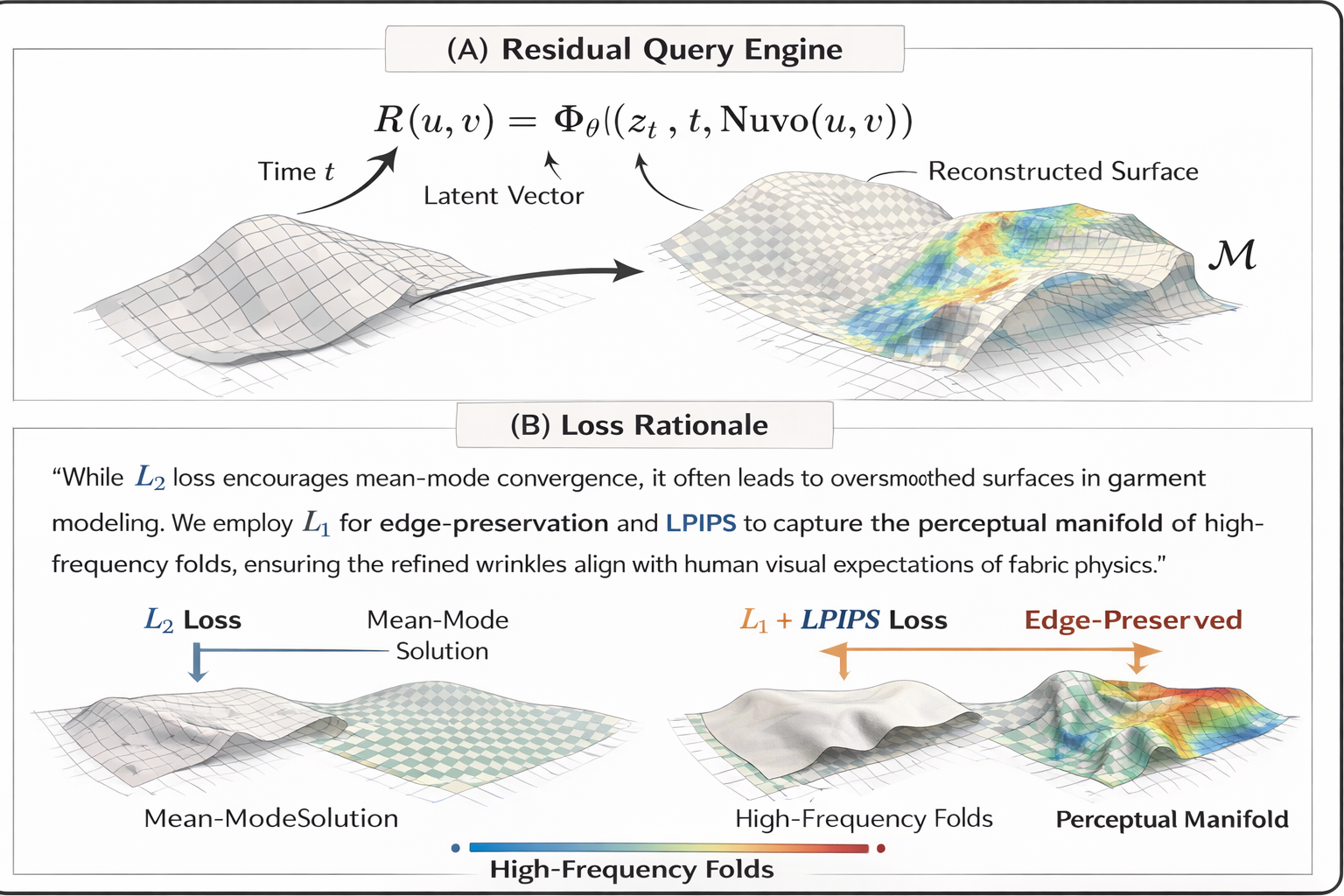
R(u,v) = Φ_θ((z_t, t, Nuvo(u,v)))
nuvo_features = diffusion_model.get_nuvo_features(points, nuvo_model)
spatial_dist = torch.norm(point_diff, dim=-1, keepdim=True) + 1e-8 <- change here for your 3D Hash value assignment
normalized_diff = residual_diff / spatial_dist <- change here

Config

• python train.py –config configs/icml.yaml –sample_idx 5 –material stiff –diffusion_steps 10

- **Stage 1** (0-5000): Nuvo only
- **Stage 2** (5000-10000): Nuvo + ND with hash assignment
num_iterations: 10000
diffusion_start_iter: 5000

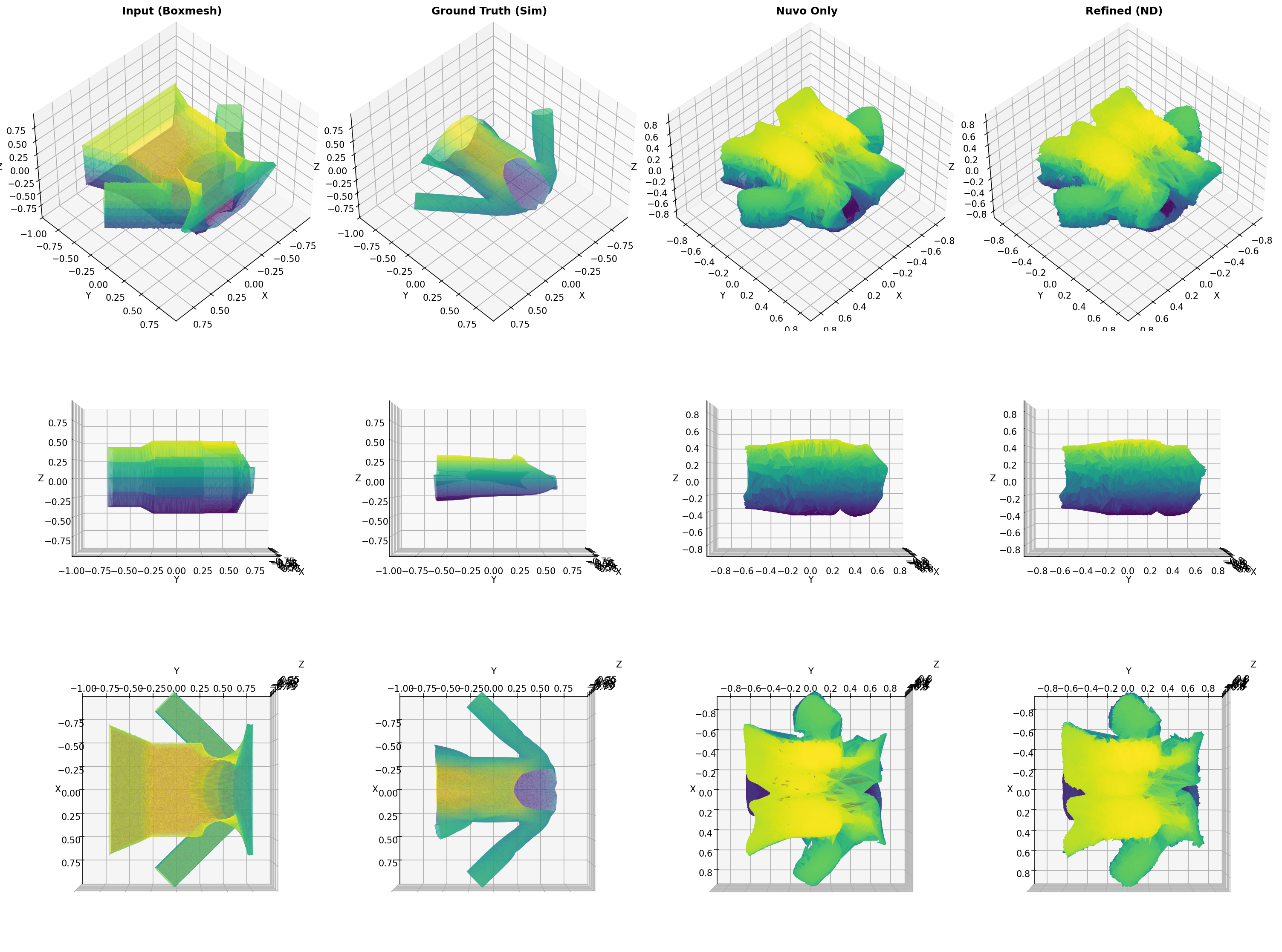
Input (Boxmesh) Details Analysis:
  Vertices: 67970
  Normal variation:
    Mean: 0.076664
    Std:  0.263265
    Max:  2.000000
  Curvature proxy:
    Mean: 104265.058453
    Std:  1197198.073828
    Max:  92199800.035140
  OK: Input (Boxmesh) has good details (mean >= 0.05)

Ground Truth (Sim) Details Analysis:
  Vertices: 67970
  Normal variation:
    Mean: 0.443511
    Std:  0.523963
    Max:  1.999905
  Curvature proxy:
    Mean: 825298.086679
    Std:  8333963.860213
    Max:  196949800.860008
  OK: Ground Truth (Sim) has good details (mean >= 0.05)

Residuals Analysis:
  Mean magnitude: 0.222847
  Std magnitude:  0.076963
  Max magnitude:  0.530114
  Min magnitude:  0.044882
  OK: Residuals are significant (mean >= 0.05)

High-frequency residuals:
  Mean: 0.087973
  Max:  0.934507
  OK: High-frequency details present

Tools

End-to-End Dataflow

Overview

• We demonstrate that, under high-performance hardware (H200) conditions, constructing a geometry-aligned discrete hash field is the optimal solution for handling high-frequency garment details compared to stacking deep MLPs.
• By defining the diffusion process within the residual hash space, we achieve 📍 per-point refinement cost does not scale with geometric complexity for complex nonlinear folds.
• three_two_three (bijective constraint): Equivalent to assert hash_map.size() == unique_points.size(). A low weight for this constraint indicates severe hash collisions, meaning multiple 3D points map to the same UV, resulting in a blurry rendering.
• cluster (clustering constraint): Equivalent to assert is_adjacent(p1, p2) == is_adjacent(hash(p1), hash(p2)). It ensures that spatially adjacent points are also close together in the hash bucket, preventing the rendering from becoming fragmented.

model:
  num_charts: 8
  use_vertex_duplication: true *https://github.com/ruiqixu37/Nuvo
-> then for the diffusion process -> It's just about tweaking details in a function space where the geometry is already aligned.
  hidden_dim: 256
  num_layers: 8

Assign Hash to your Nvidia sponsored renders

SELECT residual
FROM garment_surface
WHERE uv = (u, v);

• Nuvo is Data Indexer
• Diffusion is Error Corrector
• H200 is Hardware Accelerator

Can also add a “stitching graph consistency check”, which is essentially a Union-Find problem in graph theory, ensuring that the hash values ​​at the stitching points of two pieces eventually converge to the same value.

• By discretize the 3D space：
  • Hash function is Nuvo. It maps $P(x,y,z)$ to a specific (chart_id, u, v).
  • Key is these UV coordinates.
  • Value is the corresponding geometric residual $R$.
  • The beauty lies in avoiding all the pitfalls of high-frequency signal fitting, because the hash table itself can perfectly store high-frequency information, requiring no Fourier transform patching.
  • In academia, this is called Discrete Latent Space Alignment.

📍 Notes - Once it becomes discrete geometry, you don’t have to work on it anymore, all been solved by a large Hash Table -> let’s move on to Continuous Geometry / Signal Processing in Liver predictor

python train_demo.py --config configs/demo.yaml --sample_idx 5

Losses: Diffusion (MSE) + LPIPS
- diffusion_weight: 1.0
- lpips_weight: 0.5
- l1_weight: 0.5 (metric only)

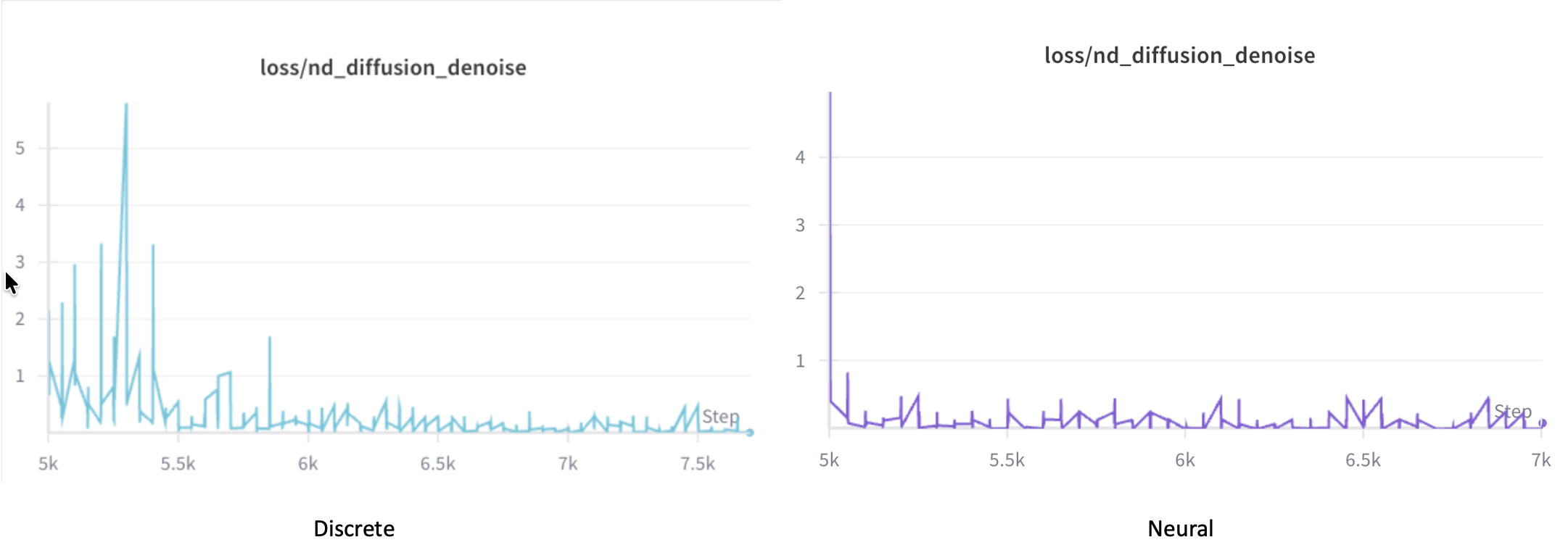
Some Over-smooth Outcome

• In LeetCode, a coordinate point is simply (x, y), the logic is very clear. However, in current computer graphics papers, the goal is to enable neural networks to optimize this point, The truth: This is essentially because MLPs (Neural Networks) are too inefficient / un-flexible, they can’t remember high-frequency details. So, people manually add “external storage” to them.

• In LeetCode, your opponent is computational complexity, at SIGGRAPH, your opponent is entropy.

  • The hash-value mindset you like (for example, Instant-NGP) is essentially a classic programmer’s counterattack. It no longer tries to understand complex geometric continuity. Instead, it says: I don’t care how complicated your surface is—I’ll just chop you up in hash space and look you up in a table
  • This approach—trading space for time, and lookup tables for computation—may have little aesthetic appeal in the eyes of mathematicians, but on an H200, it runs the fastest

Modern Hardware-aware Algorithm

• In the CPU era, algorithms aimed to reduce instruction cycles;
• In the GPU era, algorithms aim to achieve memory coalescing and avoid branch prediction.

The fundamental limitations of monocular (2D) video input

Vector Field, Probability Flow, and the Continuity Equation in Diffusion / Flow

SUMO Bridge

┌────────────────────────────┐
│ SUMO Bridge (Traffic Sim)  │
│  - Runs locally, offline   │
│  - Outputs vehicle poses & │
│    event timestamps        │
└─────────────┬──────────────┘
              │
   (Shared Memory / TCP localhost)
              │
┌─────────────▼──────────────┐
│ Unreal Engine (VR Runtime) │
│  - Renders the scene       │
│  - Receives SUMO data      │
│  - Triggers audio events   │
│  - Synchronizes pose with  │
│    HTC Vive SDK            │
└───────┬─────────┬──────────┘
        │         │
 (SteamVR API)  (Audio EXE via DP port)
        │         │
┌───────▼─────────▼──────────────┐
│ HTC Vive Headset + Controllers │
│  - IMU / Lighthouse tracking   │
│  - Controller input via        │
│    SteamVR runtime             │
└────────────────────────────────┘

In a Hardware system, there are 3 essential layers

User Feedback - If Dizzy

HTC Vive Tracking Architecture (Lighthouse System)

HTC Vive Software Stack

The Role of DP (DisplayPort)

Data Types

Physical Layers For the Data Flow

1. SUMO ↔ Unreal Engine

2. Unreal Engine ↔ HTC Vive (Headset + Controllers)

(1) Video and Audio Signals

(2) Sensor and Control Signals

Time Alignment

• Without an internet connection, there is no external time source (such as NTP or PTP). Therefore, all components must share a master clock, and every process synchronizes around it
• What happens if your master clock is the system clock
  • You can run completely offline
  • You can maintain full timestamp consistency between Unreal, the EXE, and the HMD as long as every process refers to the same local system time or the same bridge-provided clock derived from it

┌────────────────────────┐
│  C++ SyncServer        │   ← master process
│  - owns master clock   │
│  - sends {frame_idx, t}│
└────────┬───────────────┘
         │ sockets (localhost)
┌────────▼────────┐     ┌────────▼────────┐
│ Unreal Engine   │     │ SUMO Process    │
│ (Client)        │     │ (Client)        │
│ uses t, frame # │     │ uses t, frame # │
└─────────────────┘     └─────────────────┘

The essence of NTP

• To make sure that every computer (or process) in a network agrees on the same notion of time

[ SUMO Process ]
     │  Δt = 100 ms
     ▼
  "SumoCommunicationRunnable"
     │  sends {frame_id, sim_time}
     ▼
[ Local NTP / Sync Bridge ]
     │  broadcasts {sim_time, delta}
     ▼
[ Unreal Engine Runtime ]
     │
     ├── updates Actor transforms at t = sim_time
     └── triggers AudioBridge event “engine_start” @ t = sim_time
           │
           ▼
[ Audio EXE ]
     aligns its playback clock to t = sim_time

Volumetric Representation vs. NeRF vs. Gaussian Splatting

Implicit vs Explicit Representations

Geometric Shape Modeling

• 2025 - TetWeave: Isosurface Extraction using On-The-Fly Delaunay Tetrahedral Grids for Gradient-Based Mesh Optimization - Multi-view 3d reconstruction, geometric texture generation, gradient-based mesh optimization, Isosurface Representation, Fabricaible

Marching Tetrahedra on Delaunay Triangulation
(isosurface extraction on arbitrary point clouds)
                 ↓
Directional Signed Distance
(spherical harmonics; edge-aware surface accuracy)
                 ↓
Adaptive Tetrahedral Grid
(resampling where error is high; grid fits unknown surfaces)
                 ↓
Regularization Terms
(fairness + ODT loss; improve mesh quality, avoid slivers)

References

• 2025 - Single-Image 3D Human Reconstruction with 3D-Aware Diffusion Priors and Facial Enhancement
• 2025 - Find Any Part in 3D
• 2025 - Jamais Vu: Exposing the Generalization Gap in Supervised Semantic Correspondence
• 2024 - DressCode: Autoregressively Sewing and Generating Garments from TextGuidance
• 📍 2025 - AIpparel: A Multimodal Foundation Model for Digital Garments
• 2025 - TetWeave: Isosurface Extraction using On-The-Fly Delaunay Tetrahedral Grids